Martin North – Page 1026 – Digital Finance Analytics (DFA) Blog

AU$ Movements Before RBA Rate Releases Were “Normal” – ASIC

ASIC today released an update on their investigations into AU$ trading movements around the time of recent RBA target rate announcements. Whilst their investigations are ongoing, ASIC says the movements are related to liquidity positions and computer based trading, and do not indicate cases of market misconduct.

ASIC today provided an update on its investigation into the movements in the Australian dollar shortly before the Reserve Bank’s monetary policy decisions for February, March and April 2015.

The enquiry is investigating trading in the dollar in the minute prior to the RBA’s interest rate decision statement at 2.30pm.

ASIC has made extensive enquiries into the management of the information flow regarding the RBA’s interest rate decision prior to the announcement of this decision.

ASIC’s current focus is on reviewing the trading behaviour of a number of foreign exchange markets and platforms including interest rate futures markets and CFD platforms providing foreign exchange markets. Notices to produce trading information have been sent to many financial institutions and platform providers to understand the basis of the trading on these markets at the point in time of interest.

ASIC’s enquiries are ongoing as to the cause of the swings in the currency markets. Preliminary findings reveal moves in the Australian Dollar ahead of the announcement to be as a result of normal market operations in an environment of lower liquidity immediately ahead of the RBA announcement. The reduction in liquidity providers is a usual occurrence prior to announcement in all markets. Much of the trading reviewed to date was linked to position unwinds by automated trading accounts linked to risk management logic and not misconduct.

In particular, ASIC has observed liquidity being withdrawn from the market at the same moment as participants already positioned were considering their risk exposure too large ahead of the announcement and reducing their position. This lack of liquidity distorted the execution logic in the algorithms of some participant systems. This, along with a fall in trading volumes leading up to the release of key market data, means trades may have had a more pronounced impact on the price than they otherwise would.

Government Strengthens the Foreign Investment Framework

The Government today announced details of the changes which will be brought in on 1 December 2015, to clamp down on illegal foreign property purchases. Fees will be introduced for foreign investment applications. Since the measures were mooted, about 100 cases of potential illegal purchase are being investigated at the moment. For example, one case in WA involved a property of around $800,000. People have until 30th November to come forward to avoid prosecution, but will have to sell. The release follows:

The Commonwealth Government is taking action to strengthen the integrity of the foreign investment framework. Foreign investment is integral to Australia’s economy and we welcome all investment that is not contrary to our national interest. After extensive consultations on our Options Paper, we are announcing important reforms to foreign investment that will help to demonstrate that it is for our country’s benefit.

We will ensure stronger enforcement of new and existing foreign investment rules by transferring all residential real estate functions to the Australian Taxation Office. The ATO will use its data-matching systems to identify possible breaches and the Commonwealth will pursue those foreign investors who break the rules.

Australia’s foreign investment regime generally does not allow foreign investors to purchase existing residential properties. There will now be stricter penalties to make it easier to pursue foreign investors who breach the rules. Criminal penalties will be increased to $127,500 or three years imprisonment for individuals and to $637,500 for companies. Divestment orders will be supplemented by civil pecuniary penalties and infringement notices for less serious breaches.

The Government will also ensure that people who break the rules do not profit by introducing a civil penalty to capture any capital gain made on divestment of a property. Third parties who knowingly assist a foreign investor to breach the rules will also now be subject to civil and criminal penalties, including fines of $42,500 for individuals and $212,500 for companies.

Australian taxpayers will no longer foot the bill for screening foreign investment application applications. Fees will be levied on all foreign investment applications. For residential properties valued at $1 million or less, foreign investors will pay a fee of $5,000. Higher fees will apply to more expensive residential properties as well as business, agriculture and commercial real estate applications.

Australia’s foreign investment policy for residential real estate is designed to increase Australia’s housing stock, but lack of enforcement over recent years has threatened the integrity of the framework. We will enforce the rules, ensuring that all foreign investors follow the rules and don’t profit from breaking them.

The Government will introduce legislation into Parliament in the Spring Sittings to ensure that the reforms will commence on 1 December 2015.

There will also be increased scrutiny around foreign investment in agriculture and increased transparency on the levels of foreign ownership in Australia through a comprehensive land register.

Basel IV – Is More Complexity Better?

In December 2014, The Bank For International Settlements issued proposed Revisions to the Standardised Approach for credit risk for comment. It proposes an additional level of complexity to the capital calculations which are at the heart of international banking supervision. Comments on the proposals were due by 27 March 2015. These latest proposals, which have unofficially been dubbed “Basel IV”, is a continuation of the refining of the capital adequacy ratios which guide banking supervisors and relate to the standardised approach for credit risk. It forms part of broader work on reducing variability in risk-weighted asset. We want to look in detail at the proposals relating to residential real estate, because if adopted they would change the capital landscape considerably. Note this is separate from the proposal relating to the adjustment of IRB (internal model) banks. Whilst it aspires to simplify, the proposals are, to put it mildly, complex

For the main exposure classes under consideration, the key aspects of the proposals are:

Bank exposures would no longer be risk-weighted by reference to the external credit rating of the bank or of its sovereign of incorporation, but they would instead be based on a look-up table where risk weights range from 30% to 300% on the basis of two risk drivers: a capital adequacy ratio and an asset quality ratio.
Corporate exposures would no longer be risk-weighted by reference to the external credit rating of the corporate, but they would instead be based on a look-up table where risk weights range from 60% to 300% on the basis of two risk drivers: revenue and leverage. Further, risk sensitivity would be increased by introducing a specific treatment for specialised lending.
The retail category would be enhanced by tightening the criteria to qualify for the 75% preferential risk weight, and by introducing a fallback subcategory for exposures that do not meet the criteria.
Exposures secured by residential real estate would no longer receive a 35% risk weight. Instead, risk weights would be determined according to a look-up table where risk weights range from 25% to 100% on the basis of two risk drivers: loan-to-value and debt-service coverage ratios.
Exposures secured by commercial real estate are subject to further consideration where two options currently envisaged are: (a) treating them as unsecured exposures to the counterparty, with a national discretion for a preferential risk weight under certain conditions; or (b) determining the risk weight according to a look-up table where risk weights range from 75% to 120% on the basis of the loan-to-value ratio.
The credit risk mitigation framework would be amended by reducing the number of approaches, recalibrating supervisory haircuts, and updating corporate guarantor eligibility criteria.

Real Estate Capital Calculation Proposals

The recent financial crisis has demonstrated that the current treatment is not sufficiently risk-sensitive and that its calibration is not always prudent. In order to increase the risk sensitivity of real estate exposures, the Committee proposes to introduce two specialised lending categories linked to real estate (under the corporate exposure category) and specific operational requirements for real estate collateral to qualify the exposures for the real estate categories.

Currently the standardised approach contains two exposure categories in which the risk-weight treatment is based on the collateral provided to secure the relevant exposure, rather than on the counterparty of that exposure. These are exposures secured by residential real estate and exposures secured by commercial real estate. Currently, these categories receive risk weights of 35% and 100%, respectively, with a national discretion to allow a preferential risk weight under certain strict conditions in the case of commercial real estate.

Residential Owner Occupied Real Estate

In order to qualify for the risk-weight treatment of a residential real estate exposure, the property securing the mortgage must meet the following operational requirements:

Finished property: the property securing a mortgage must be fully completed. Subject to national discretion, supervisors may apply the risk-weight treatment for loans to individuals that are secured by an unfinished property, provided the loan is for a one to four family residential housing unit.
Legal enforceability: any claim (including the mortgage, charge or other security interest) on the property taken must be legally enforceable in all relevant jurisdictions. The collateral agreement and the legal process underpinning the collateral must be such that they provide for the bank to realise the value of the collateral within a reasonable time frame.
Prudent value of property: the property must be valued for determining the value in the LTV ratio. Moreover, the value of the property must not be materially dependent on the performance of the borrower. The valuation must be appraised independently using prudently conservative valuation criteria and supported by adequate appraisal documentation.

The current standardised approach applies a 35% risk weight to all exposures secured by mortgage on residential property, regardless of whether the property is owner-occupied, provided that there is a substantial margin of additional security over the amount of the loan based on strict valuation rules. Such an approach lacks risk sensitivity: a 35% risk weight may be too high for some exposures and too low for others. Additionally, there is a lack of comparability across jurisdictions as to how great a margin of additional security is required to achieve the 35% risk weight.

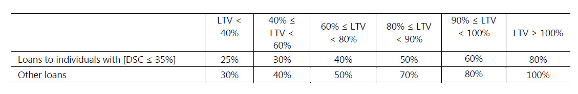
In order to increase risk sensitivity and harmonise global standards in this exposure category, the Committee proposes to introduce a table of risk weights ranging from 25% to 100% based on the loan-to-value (LTV) ratio. The Committee proposes that the risk weights derived from the table be applied to the full exposure amount (ie without tranching the exposure across different LTV buckets).

The Committee believes that the LTV ratio is the most appropriate risk driver in this exposure category as experience has shown that the lower the outstanding loan amount relative to the value of the residential real estate collateral, the lower the loss incurred in the event of a default. Furthermore, data suggest that the lower the outstanding loan amount relative to the value of the residential real estate collateral, the less likely the borrower is to default. For the purposes of calculating capital requirements, the value of the property (ie the denominator of the LTV ratio) should be measured in a prudent way. Further, to dampen the effect of cyclicality in housing values, the Committee is considering requiring the value of the property to be kept constant at the value calculated at origination. Thus, the LTV ratio would be updated only as the loan balance (ie the numerator) changes.

The LTV ratio is defined as the total amount of the loan divided by the value of the property. For regulatory capital purposes, when calculating the LTV ratio, the value of the property will be kept constant at the value measured at origination, unless an extraordinary, idiosyncratic event occurs resulting in a permanent reduction of the property value. Modifications made to the property that unequivocally increase its value could also be considered in the LTV. The total amount of the loan must include the outstanding loan amount and any undrawn committed amount of the mortgage loan. The loan amount must be calculated gross of any provisions and other risk mitigants, and it must include all other loans secured with liens of equal or higher ranking than the bank’s lien securing the loan. If there is insufficient information for ascertaining the ranking of the other liens, the bank should assume that these liens rank pari passu with the lien securing the loan.

In addition, as mortgage loans on residential properties granted to individuals account for a material proportion of banks’ residential real estate portfolios, to further increase the risk sensitivity of the approach, the Committee is considering taking into account the borrower’s ability to service the mortgage, a proxy for which could be the debt service coverage (DSC) ratio. Exposures to individuals could receive preferential risk weights as long as they conform to certain requirement(s), such as a ‘low’ DSC ratio. This ratio could be defined on the basis of available income ‘net’ of taxes. The DSC ratio would be used as a binary indicator of the likelihood of loan repayment, ie loans to individuals with a DSC ratio below a certain threshold would qualify for preferential risk weights. The threshold could be set at 35%, in line with observed common practice in several jurisdictions. Given the difficulty in obtaining updated borrower income information once a loan has been funded, and also given concerns about introducing cyclicality in capital requirements, the Committee is considering whether the DSC ratio should be measured only at loan origination (and not updated) for regulatory capital purposes.

The DSC ratio is defined as the ratio of debt service payments (including principal and interest) relative to the borrower’s total income over a given period (eg on a monthly or yearly basis). The DSC ratio is defined using net income (ie after taxes) in order to focus on freely disposable income. The DSC ratio must be prudently calculated in accordance with the following requirements:

Debt service amount: the calculation must take into account all of the borrower’s financial obligations that are known to the bank. At loan origination, all known financial obligations must be ascertained, documented and taken into account in calculating the borrower’s debt service amount. In addition to requiring borrowers to declare all such obligations, banks should perform adequate checks and enquiries, including information available from credit bureaus and credit reference agencies.
Total income: income should be ascertained and well documented at loan origination. Total income must be net of taxes and prudently calculated, including a conservative assessment of the borrower’s stable income and without providing any recognition to rental income derived from the property collateral. To ensure the debt service is prudently calculated, the bank should take into account any probable upward adjustment in the debt service payment. For instance, the loan’s interest rate should (for this purpose) be increased by a prudent margin to anticipate future interest rate rises where its current level is significantly below the loan’s long-term level. In addition, any temporary relief on repayment must not be taken into account for purposes of the debt service amount calculation.

Notwithstanding the definitions of the DSC and LTV ratios, banks must, on an ongoing basis, have a comprehensive understanding of the risk characteristics of their residential real estate portfolio.

The risk weight applicable to the full exposure amount will be assigned, as determined by the table below, according to the exposure’s loan-to-value (LTV) ratio, and in the case of exposures to individuals, also taking into account the debt service coverage (DSC) ratio. Banks should not tranche their exposures across different LTV buckets; the applicable risk weight will apply to the full exposure amount. A bank that does not have the necessary LTV information for a given residential real estate exposures must apply a 100% risk weight to such an exposure.

Some points to note.

Differences in real estate markets, as well as different underwriting practices and regulations across jurisdictions make it difficult to define thresholds for the proposed risk drivers that are meaningful in all countries.
Another concern is that the proposal uses risk drivers prudently measured at origination. This is mainly to dampen the effect of cyclicality in housing values (in the case of LTV ratios) and to reduce regulatory burden (in the case of DSC ratios). The downside is that both risk drivers can become less meaningful over time, especially in the case of DSC ratios, which can change dramatically after the loan has been granted.
The DSC ratio is defined using net income (ie after taxes) in order to focus on freely disposable income. That said, the Committee recognises that differences in tax regimes and social benefits in different jurisdictions make the concept of ‘available income’ difficult to define and there are concerns that the proposed definition might not be reflective of the borrower’s ability to repay a loan. Further, the level at which the DSC threshold ratio has been set might not be appropriate for all borrowers (eg high income) or types of loans (eg those with short amortisation periods). Therefore the Committee will explore whether using either a different definition of the DSC ratio (eg using gross income, before taxes) or any other indicator, such as a debt-to-income ratio, could better reflect the borrower’s ability to service the mortgage.
There are no specific proposal to treat loans that are past-due for more than 90 days.

Investment Loans

Bearing in mind that 35% of all loans are for investment purposes in Australia, the proposals relating to loans for investment purposes are important. So how will they be treated under Basel 4?

There are a number of pointers in the proposals, though its not totally clear in our view. First, we think the proposals would apply to separate loans where repayment is predicated on income generated by the property securing the mortgage, i.e. investment loans rather than a normal loans where the mortgage is linked directly to the underlying capacity of the borrower to repay the debt from other sources. Such loans might fall into a special commercial real estate category, specialist lending category, or a fall back to the unsecured category, each with different sets of capital weights.

The Committee proposes that any exposure secured with real estate that exhibits all of the characteristics set out in the specialised lending category should be treated for regulatory capital purposes as income-producing real estate or as land acquisition, development and construction finance as the case may be, rather than as exposures secured by real estate. Any non-specialised lending exposure that is secured by real estate but does not satisfy the operational requirements should be treated for regulatory capital purposes as an unsecured exposure, either as a corporate exposure or other retail exposure, as appropriate.

Specialised lending exposure, would be defined so if all the following characteristics, either in legal form or economic substance were met:

The exposure is typically to an entity (often a special purpose entity (SPE)) that was created specifically to finance and/or operate physical assets;
The borrowing entity has few or no other material assets or activities, and therefore little or no independent capacity to repay the obligation, apart from the income that it receives from the asset(s) being financed;
The terms of the obligation give the lender a substantial degree of control over the asset(s) and the income that it generates; and
As a result of the preceding factors, the primary source of repayment of the obligation is the income generated by the asset(s), rather than the independent capacity of a broader commercial enterprise.

On the other hand, in order to qualify as a commercial real estate exposure, the property securing the mortgage must meet the same operational requirements as for residential real estate. If the loan is a commercial real estate category, the risk weight applicable to the full exposure amount will be assigned according to the exposure’s loan-to-value (LTV) ratio, as determined in the table below. Banks should not tranche their exposures across different LTV buckets; the applicable risk weight will apply to the full exposure amount. A bank that does not have the necessary LTV information for a given commercial real estate exposure must apply a 120% risk weight.
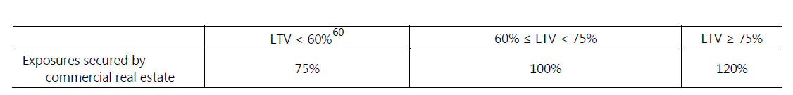
LTVNote, if this LTV refers to market value, the threshold should be set at a lower level: eg 50%.

Where the requirements are not met, the exposure will be considered unsecured and treated according to the counterparty, ie as “corporate” exposure or as “other retail”. However, in exceptional circumstances for well developed and long established markets, exposures secured by mortgages on office and/or multipurpose commercial premises and/or multi-tenanted commercial premises may be risk-weighted at [50%] for the tranche of the loan that does not exceed 60% of the loan to value ratio. This exceptional treatment will be subject to very strict conditions, in particular:

the exposure does not meet the criteria to be considered specialised lending
the risk of loan repayment must not be materially dependent upon the performance of, or income generated by, the property securing the mortgage, but rather on the underlying capacity of the borrower to repay the debt from other sources
the property securing the mortgage must meet the same operational requirements as for residential real estate
two tests must be fulfilled, namely that (i) losses stemming from commercial real estate lending up to the lower of 50% of the market value or 60% of loan-to value (LTV) based on mortgage-lending-value (MLV) must not exceed 0.3% of the outstanding loans in any given year; and that (ii) overall losses stemming from commercial real estate lending must not exceed 0.5% of the outstanding loans in any given year. This is, if either of these tests is not satisfied in a given year, the eligibility to use this treatment will cease and the original eligibility criteria would need to be satisfied again before it could be applied in the future. Countries applying such a treatment must publicly disclose that these and other additional conditions (that are available from the Basel Committee Secretariat) are met. When claims benefiting from such exceptional treatment have fallen past-due, they will be risk-weighted at [100%].

Implications and Consequences

We should make the point, these are proposals, and subject to change. But it would mean that banks using the standard approach to capital could no longer just go with a 35% weighting, rather they will need to segment the book based on LTV and servicability at a loan by loan level. Investment loans may become more complex and demand higher capital weighting. The required data may be available, as part of the loan origination process, but additional processes and costs will be incurred, and it appears net-net capital buffers will be raised for most players. The capital would be determined using two risk drivers: loan-to-value and debt-service coverage ratios with risk weights ranging from 25 percent to 100 percent. Investment loans may require different treatment, (and the RBNZ discussion paper recently issued may be relevant here, where investment loans are handled on a different basis.)

Finally, a word about those banks on IRB. Currently, under their internal models, they are sitting on an average weighting of around 17% (compared with 35% for standard banks). There are proposals to lift the floor to 20% minimum, and the FSI Inquiry recommend higher. Indeed, Murray called for the big banks to lift the average mortgage risk weighting to a range of 25% to 30%. This would bring them closer to the average mortgage risk weighting used by Australia’s regional banks and credit unions, though as described above, these, in turn, may change. Incidentally, the Bank of England thinks 35% is a good target. Basel 4 will also reduce the variance between standardised banks and those using their own models by requiring the internal models not to deviate from the RWA number in the standardised model by a certain amount: the so-called “capital floor”.

Interestingly the US is focussing on an additional measure, The Tier 1 Common measure, which is unweighted assets to capital, and has set a floor of 5%, or more. The Major Banks in Australia carry real, or non-risk-weighted, equity capital of just 3.7% of assets. Some banks are leveraged over seventy times the equity capital to loans, which is scarily high, but then the RBA (aka the tax payer) would bail them out if they get into trouble, so that’s OK (or not). This means that just $1.70 in assets will now support a $100 loan.

We wonder if the ever more complex models being proposed by Basel are missing the point. Maybe we should be going for something simpler. Many banks of course have invested big in advanced models to squeeze the capital lemon as hard as they can. But stepping back we need approaches which allow greater ability to compare across banks, and more transparent disclosure so we can see where the true risks lay. Certainly capital buffers should be lifted, but we suspect Basel 4, despite the best of intentions, is going down the wrong alley.

Foreign Property Investment Up – FIRB

The Foreign Investment Review Board recently published their annual report for 2013-2014. Whilst we question whether they capture the full picture, the report shows that real estate and services related applications accounted for around 76 per cent of the value of approvals in 2013-14. China was the largest investor in 2013-14 in terms of the value of all approvals (17 per cent of the total value), followed by the United States and Canada. Three (yes three!) proposals were rejected in the year.

In 2013-14, 24,102 proposals received foreign investment approval, compared with 12,731 in 2012-13. The real estate sector had a significant increase in approvals with 23,428 approvals in 2013-14,compared with 12,025 approvals in 2012-13.

Approvals in 2013-14 were given for $167.4 billion of proposed investment. This represented a 23.4 per cent increase on the $135.7 billion in proposed investment approved in 2012-13. In real estate, approved proposed investment was $74.6 billion in 2013-14, compared with $51.9 billion in 2012-13. Proposed investment in commercial real estate increased, from $34.8 billion in 2012-13 to $39.9 billion in 2013-14. Proposed investment in residential real estate also increased, from $17.2 billion in 2012-13 to $34.7 billion in 2013-14.
In 2013-14, three proposals were rejected (compared with no rejected proposals in 2012-13). Of the three proposals rejected, two related to residential real estate and the other related to the rejection in November 2013 of Archer Daniel Midlands Company’s proposed takeover of GrainCorp Limited.

The real estate sector was the largest destination by value, with approvals in 2013-14 of $74.6 billion (an increase of $22.7 billion from 2012-13). In 2013-14, the other major sectors were: services (excluding tourism), with approved proposed investment of $53.4 billion (an increase of $27.5 billion); and mineral exploration and development, with approved proposed investment of $22.4 billion (a decrease of $23.1 billion).

Real Estate accounted for 44.6% ot the total value. Here is the more detailed breakdown.

For the first time China ($27.7 billion) was the largest source country for approved proposed investment in 2013-14, overtaking the United States ($17.5 billion). Other major source countries of approved proposed investment in 2013-14 were Canada ($15.4 billion), Malaysia ($7.2 billion) and Singapore ($7.1 billion).

On 25 February 2015, the Government released an options paper on Strengthening Australia’s Foreign Investment Framework. The paper is available on the Treasury website. The Government has announced that a $15 million cumulative threshold will apply to acquisitions of interests in agricultural land from 1 March 2015. More announcements are expected very soon on how the regime will be reinforced, with fines for potential investors who flout the rules, professionals who assist them, and rules to stop investors from profiting from any potential capital appreciation if they are found out, and forced to sell.

Can Indebtedness and Interest Rates Both Increase?

In FitchRating’s latest Global Perspective, James McCormack, Fitch’s Global Head of Sovereign Ratings highlights the dilemma facing the US where rates are low and debt is high. What happens when interest rates rise? Given that both household and corporate debt levels are much higher now, the potential exists for a much more negative impact in terms of debt sustainability and economic performance.

Private sector deleveraging has been a critical feature of the post-crisis US economic recovery, and will remain an important consideration for growth and stability as interest rates move higher. Borrowers have benefited from a more-than 30-year trend of falling rates, but the eventual reversal will test the degree to which private sector balance sheets have been strengthened in the post crisis period. With debt levels still high by historical standards, higher interest rates may have a pronounced impact on growth in the period ahead.

A Cycle Ends: Meaningful Deleveraging

The increase in household debt by 30 percentage points of GDP between 2000 and 2008 was unprecedented, as has been the subsequent deleveraging (see chart 1).

The previous 30 percentage point increase took more than 40 years, and there had never been a meaningful deleveraging prior to 2009. At end-2014, household debt was back to its 2002 level as a share of GDP, and below its 2008 peak in nominal terms. A similar, though less marked, pattern is evident in the corporate sector, unlike in previous credit cycles when corporate debt levels were more volatile than those of households. Corporate debt is now lower than in 2009 as a share of GDP, but 12% higher than the pre-crisis peak in nominal terms.

The Long View: Lower Rates Allowed for Higher Debt

Taking a much longer view, even accounting for post-crisis reductions, household and corporate debt levels have trended higher since the early 1950s (when data became available). Moreover, it is widely accepted – if not explicitly acknowledged – that a continuation of this trend is a sign the US economy is getting back to “normal”. The resumption of private sector credit growth on the back of improved balance sheets is a big part of the narrative of the US recovery, and a meaningful difference with conditions in the Eurozone. Historical interest rate developments provide insight to the steady run-up in US debt, and are a basis of concern looking forward. Both nominal and real medium-term interest rates (approximated by 10-year US Treasury yields) have been falling since the early 1980s. Over the same period, there have been matching declines in effective interest rates faced by the household and corporate sectors (see chart 2).

Effective rates are calculated using BEA data on Interest Paid and Received by Sector, and Flow of Funds data on outstanding debt stocks. Critically, for the last 30 years, falling interest rates have offset the effects of higher debt levels to keep interest service ratios manageable (see chart 3).

There is a strong historical relationship between US economic growth and interest rates in both real and nominal terms. Over the last 50 years real GDP growth and 10-year US Treasury yields (using the GDP deflator) averaged 3.1% and 3.0%, respectively. In nominal terms they averaged 6.7% and 6.6%. On this basis, with 10-year Treasuries yielding less than 2%, they appear low by historical standards. Current conditions are certainly not unique. There have been periods when 10-year Treasury yields were consistently lower than economic growth. The last episode was the mid-2000s, when a global savings glut led to what Alan Greenspan described as a “conundrum”, whereby increases in the Fed Fund rate from 2004 were not matched by 10-year yields. With reasonably strong US growth at the time, households and corporates responded as might be expected – they borrowed more. Private credit growth subsequently outpaced nominal GDP growth and was one of the contributing factors of the global financial crisis.

The critical question is what will happen to 10-year Treasury yields and the effective interest rates faced by the corporate and household sectors as monetary policy is tightened in the current cycle? With smaller current account surpluses in Asia and among Middle East oil exporters, it seems less probable that a global savings glut will continue to hold US rates down. Despite the deleveraging that began in 2009, neither the household nor corporate sector is particularly well placed for a higher interest rate environment. Household interest payments as a share of GDP are now at the same level as the mid-1970s, when debt was lower by 35 percentage points of GDP. Corporate sector debt has increased by less, but interest payments are also at mid-1970s levels. It appears that for the first time since the early 1980s, the outlook for the US economy may be characterised by simultaneous increases in debt levels and effective interest rates. The difference now, however, is household and corporate debt levels are much higher, suggesting the potential for a much more negative impact in terms of debt sustainability and economic performance.

Home Prices Higher In April – CoreLogic RP Data

CoreLogic RP Data April Home Value Index results confirmed that values across Australia’s combined capital cities increased by 0.8 per cent in April 2015, down from a 1.4 per cent month on month increase in March. Overall dwelling values shifted higher over the past month across every capital city except Canberra where values showed a 1.5 per cent drop over the month.

According to the April Home Value results, capital city dwelling values have been trending higher over the past 35 months, recording a cumulative increase of 25.3 per cent between the end of May 2012 and April 2015. While the combined capitals trend of dwelling value growth has been substantial, the rate of growth across the Sydney housing market stands head and shoulders above the other capital cities over the cycle to date. Sydney dwelling values are now 40.2 per cent higher relative to the May 2012 trough. If you factor in the previous 2009/10 phase of growth, Sydney values are now up 65.4 per cent post GFC. Melbourne is the only other capital city that comes close to this measure where dwelling values are 52.3 per cent higher post GFC. The next highest rate of growth is Darwin where values have moved 26.5 per cent higher, followed by Canberra (19.8%), Perth (15.2%), Adelaide (12.2%), Brisbane (8.0%) and Hobart (1.2%). The rate of growth in Perth and Darwin has slowed substantially in line with the wind down of major infrastructure projects associated with the resources sector and the housing market in Canberra has also softened post federal election.

The performance of houses versus apartments has shown some interesting trends of late. Detached homes are continuing to outperform the multi-unit sector, with capital city house values up 8.3 per cent over the past year while unit values have risen by a lower 5.6 per cent. This trend is more noticeable in the key growth markets of Sydney and Melbourne. Sydney house values are up 15.5 per cent over the past year while unit values have risen by 9.7 per cent. The over-performance of houses compared with units is more apparent in Melbourne where house values are 7.6 per cent higher over the year compared with a growth rate of just 1.9 per cent across the unit market. A similar trend is evident across most of the capital cities and can likely be attributed to the higher supply levels in the apartment markets which are keeping a lid on the rate of capital gain.

Most other housing market indicators remain strong. Auction clearance rates have surged to new record highs after the February rate cut and have trended slightly higher over the final two weeks of April. Additionally, the number of homes being advertised for sale has been trending lower, particularly in Sydney where listing numbers are now lower than the number of properties being advertised for sale in Melbourne, Brisbane and Perth. The short supply of advertised homes in Sydney is likely to be one of the key factors driving local dwelling values higher, with buyers pressured to make a purchase decision quickly with minimal negotiation on asking prices due to few alternative housing options available for sale.

The performance of the housing market is increasingly varied across the capital cities. Sydney is continuing to dominate the headlines with such a high rate of capital gain, while Melbourne is also showing a solid performance. At the other end of the spectrum, Perth, Darwin, Hobart and Canberra are showing weaker results while Brisbane and Adelaide and are roughly keeping pace with inflation. In fact, outside of Sydney and Melbourne, the next highest rate of annual capital gain can be found in Brisbane where dwelling values are up a comparatively paltry 2.2 per cent.

Residential Building Hotspots – HIA

The latest HIA/ACI Population and Residential Building Hotspots Report shows Western Australia again dominating the latest league table, with Victoria and New South Wales also strongly represented. Nationally, a “Hotspot” is defined as a local area where population growth exceeds the national rate and where the value of residential building work approved is in excess of $100 million. Local areas featuring on the Building Momentum shortlist have demonstrated consistently strong rates of population growth in recent years in addition to an increase in the estimated value of new home building work approved in 2014/15.

Six of the top twenty Hotspots were in Western Australia, followed by Victoria with five and New South Wales with four. For a second consecutive year, it was the Australian Capital Territory that was home to Australia’s number one building and population Hotspot – the territory’s South West area. Second place was the Northern Territory’s Palmerston South area. The ACT was also home to Australia’s number three Hotspot, the suburb of Crace.

This year’s Hotspots report also provides a Building Momentum shortlist which identifies a number of regions where further upward momentum in building activity is set to occur in 2015. Strong potential is evident for local areas in NSW in particular, while WA and Victoria also feature quite broadly. In contrast, the ACT does not feature on this shortlist, signalling that the experience of recent years – where a number of ACT areas have been strongly represented among the Nation’s Top 20 Hotspots – is unlikely to be replicated next year.

Length of Zero Interest Rate Policy Reflects Diminished Fundamentals – Moody’s

According to Moody’s, recently markets discovered that there was only a limited speculative demand for 10-year European government bonds yielding less than 1%. Unless forced to do so by an investment mandate, it’s highly unlikely that many long-term investors had been loading up on European government debt yielding less than 1%. Despite their latest climb, European government bond yields remained low compared to what otherwise might be inferred from fundamental drivers excluding European Central Bank (ECB) demand. ECB purchases have been substantial and are scheduled to be so. For example, the ECB still intends to purchase another one trillion euro of European bonds by the autumn of 2016.

Over the past week, the 10-year German government bond yield rose by 22 bp to 0.38%. In near lock step fashion, the 10-year US Treasury yield increased by 19 bp to 2.10%. The unexpected rise by Treasury bond yields helped to trigger an accompanying 0.9% drop by the market value of US common stock.

We still hold that the forthcoming upswing by US bond yields will more closely resemble a mild rise, as opposed to a jarring lift-off. Though financial markets are likely to overreact to the first convincing hint of a higher fed funds rate, the record shows that the market value of US common stock does not peak until several years after the initial rate hike. Yes, payrolls are growing, but the quality of new jobs may be lacking, according to the subpar growth of employee compensation and below-trend income expectations. Thus, the reaction of household expenditures, including home sales, to the expansion of payrolls and still extraordinarily low mortgage yields falls considerably short of what occurred during previous business cycle upturns. In turn, the upside for Treasury bond yields is limited. The 10-year US Treasury yield is likely to spend 2015’s final quarter in a range that is no greater than 2.25% to 2.50%.

When the federal funds rate target was first lowered to its current range of 0.00% to 0.25% in December 2008, nobody dared to predict that this record low target would hold well into 2015. Few, if any, appreciated the extent to which the drivers of expenditures growth had been weakened not only by a diminution of business and household credit quality, but also by heightened global competition and an aging population. Three overlapping and unprecedented episodes of quantitative easing have made the length of the nearly 6.5year stay by the Fed’s zero interest rate policy all the more remarkable. Neither the Fed’s $3.8 trillion net purchase of bonds since mid-2008 nor roughly $800 billion of fiscal stimulus was able to spur expenditures by enough to allow for the removal of an ultra-low fed funds rate target.
In stark contrast, fed funds’ previous bottom of 1% in 2003-2004 lasted for only 12 months. And when fed funds troughed at the 3% during late 1992 into early 1994, its duration was slightly longer at 17 months. The US economy’s decidedly positive response to each earlier bottoming of fed funds helps to explain their much shorter durations.

Long-term growth slows markedly

Amazingly, despite humongous monetary stimulus, as well as considerable fiscal stimulus, the moving yearlong sum of real GDP has grown by only 2.2% annualized since the Great Recession ended in June 2009. For comparably measured serial comparisons, 23 quarters following the expiry of the three downturns prior to the Great Recession, the average annualized rates of real GDP growth were 2.9% as of Q3-2007, 3.4% as of Q4-1996, and 4.8% as of Q3-1988. The downshifting of the average annual rate of growth by the 23rd quarter of an upturn lends credibility to the secular deceleration argument. If there is any good news it may be that the prolonged deceleration of US economic growth may be bottoming out. That being said, Q1-2015’s lower than expected estimate of real GDP increases the likelihood that 2015 will be the 10th straight year for which the annual rate of US economic growth failed to reach 3%. Such a stretch lacks recent precedent.

US real GDP will probably average a 1.5% annualized increase during the 10-years-ended 2015. Previous 10year average annualized rates of real GDP growth averaged 3.4% as of 2005, 3.0% as of 1995, and 3.5% as of 1985. Beginning and concluding with the spans-ended 1957 through 2007, the 10-year average annualized rate of real GDP growth averaged 3.4%. Most baby boomers will not live long enough to observe another average annual growth rate of at least 3% over a 10-year span.

Corporate credit heeds the diminished efficacy of stimulus

The corporate credit market is well aware of how so much monetary and fiscal stimulus supplied so little lift to business activity. In turn, credit spreads are wider than otherwise given a benign default outlook, partly because of a loss of confidence in the ability of policy actions to quickly spur expenditures out of a macroeconomic slump. In the event an adverse shock rattles the US economy, just how effective would additional monetary stimulus be at reviving growth?

Moreover, a still elevated ratio of US government debt to GDP might delay the implementation of fiscal policy by a Congress that remains skeptical of the effectiveness of increased government spending and a Presidency that is adverse to tax cuts. Also, even if Washington were to agree on fiscal stimulus, foreign investors, who now hold 47% of outstanding US Treasury debt, may be unwilling to take on more obligations of the US government unless compensated in the form of higher US Treasury bond yields. In all likelihood, an accompanying rise by private-sector borrowing costs would reduce the lift supplied by fiscal stimulus.

RBNZ Bulletin Covers Capital Markets

The New Zealand Reserve Bank today published an article in the Reserve Bank Bulletin that describes New Zealand’s capital markets, and the role they play in the functioning of financial markets and the real economy. The article is quite comprehensive, and worth reading becasue it describes the financial instruments and market participants involved, and analyses a unique dataset to provide some detail on the size of both the bond and equity markets, which together comprise local capital markets. We summarise some of the discussion.

Capital markets are the part of the financial system that involve buying and selling long-term securities – both debt (bonds) and equity instruments. Capital markets are used to fund investment or to facilitate takeovers, and to provide risk mitigation (for example via derivatives) and diversification. There is no strict definition of ‘long-term’; Potter (1995) defines capital market instruments as having a maturity of greater than one year, and we retain this classification here, noting that capital market instruments may also have no maturity date (as in the case of perpetual bonds or equity). This article further classifies the domestic capital market as all resident entities issuing into the local economy in New Zealand dollars (NZD) . The article also touches on resident entities issuing bonds offshore, and non-resident entities issuing into New Zealand in NZD.New Zealand’s capital markets are an integral part of the domestic financial system. The previous Reserve Bank Bulletin articles describing New Zealand’s capital markets were published 20 years ago. The landscape has changed dramatically since then – local capital markets have grown substantially, although remain small compared with those in many other advanced economies.

The Reserve Bank has a wide-ranging interest in New Zealand’s capital markets. The Financial Stability Report (FSR), for example, reports on the soundness and efficiency of the financial system, including capital markets. Capital markets that function effectively are important for the way monetary policy affects the wider economy. The Reserve Bank’s prudential regulation of financial institutions can also influence the type and nature of capital market instruments that develop in the local market.

Section two of the article describes capital markets in general, and defines New Zealand’s capital markets in a global context. The instruments and players involved are explained. Section three discusses why capital markets are important for any economy, while section four highlights the Reserve Bank’s interest in capital markets. Section five describes New Zealand’s capital markets and uses a unique dataset to provide detail on the size of the non-government bond market in particular. Section six notes developments since the 2009 Capital Markets Taskforce review.

One interesting piece of data relates to bond issuance. The total amount of bonds outstanding in the local market (excluding Kauris) has more than doubled since 2007 in nominal terms, rising from just over $50 billion (30 percent of GDP) at the start of 2007 to $121 billion. More than two-thirds of this rise is due to an increase in central government debt, while nearly 20 percent of the increase represents bond issuance by banks. The increase in government bond issuance is linked to the shift from fiscal surpluses to deficits during the Global Financial Crisis (GFC), and further issuance following the Christchurch earthquakes.

New Zealand banks increased their issuance of long-term debt sharply in the immediate post-GFC period. This followed from a number of changes in the global environment, including the risk of a negative credit rating from international rating agencies stemming from a reliance on short-term funding, a lack of global liquidity, and a cessation of some wholesale funding markets during the depth of the GFC (increasing the risk of a failure to roll over upcoming funding needs). In addition, New Zealand registered banks are now required by the Reserve Bank to raise a greater proportion of funding that is likely to remain in place for at least one year, as part of the prudential liquidity policy introduced in 2009. The Reserve Bank’s prudential liquidity policy was implemented to reduce the risk posed to New Zealand’s banking system by an overreliance on short-term wholesale market funding.

As at October 2014, the New Zealand (central) government sector had issued 61 percent of New Zealand’s bonds outstanding (figure 6). By comparison, the share of the local government sector was 8.5 percent, with 18.5 percent issued by banks or other financial institutions and 9 percent by non-financial corporates. SOEs comprise the remaining 3 percent. This breakdown has changed markedly since 2007; as previously noted, central government debt makes up a much larger share today, while the proportion of non-financial corporate bonds has fallen from 19 percent to its current level of 9 percent of the total. Although the nominal amount of bonds outstanding has increased for all sectors, nonfinancial corporate bonds have decreased as a share of GDP, falling from 5.7 percent to 4.5 percent currently (possibly reflecting weaker overall demand for business credit in the past five years). Note that figure 6 does not include bonds issued by New Zealand entities in offshore markets; if included, the share of government bonds would decrease.

Looking ahead, New Zealand’s equity and bond markets have grown in size and depth in recent years. Despite this, the size of New Zealand’s capital markets remains small and underdeveloped by international standards, while the banking system continues to dominate funding for New Zealand firms. On the one hand, the relatively small size of New Zealand’s capital markets might simply reflect the small size of the economy: some economies simply lack scale to support a flourishing capital market.

Laeven (2014) argues that, “in an increasingly globalised world, not every country needs to develop a fully-fledged physical capital market at home. The optimal balance between local capital market development and integration in global capital markets will depend on country circumstances, such as economic size and stage of development” (p.19). As noted in this article, larger New Zealand corporates already have access to global markets – both public debt markets and private placements.

On the other hand, many believe that further development of both equity and bond markets in New Zealand would help to underpin economic growth (CMD Taskforce, 2009). Indeed, capital market activity over the past few years has been heavily influenced by a wide range of continuing regulatory and policy initiatives to support New Zealand’s equity and bond markets. Looking ahead, the growth of KiwiSaver scheme funds and the recent partial privatisation of SOEs could add further depth and liquidity to the domestic equity market, and in turn increase international interest and participation. In addition, the development of an alternative public growth market, introduced last year by the NZX, could help to encourage more SMEs to raise funds via public listing (by offering lower compliance costs). Other policy and regulatory initiatives including formalising crowd funding via crowd funding licences issued by the FMA, could further serve to reduce capital-raising costs for small firms. That said, most of the regulatory initiatives are very recent, and at this point, it is difficult to assess how much difference these changes will make over the longer term

BIS On Financial Regulation

Interesting panel remarks at the IMF conference “Rethinking macro policy III: progress or confusion?” by Jaime Caruana, General Manager, Bank for International Settlements in Washington DC. The comments were entitled “The international monetary and financial system:eliminating the blind spot”.

Introduction

Thank you for inviting me to discuss the international monetary and financial system (IMFS) at this engaging conference. The design of international arrangements suitable for the global economy is a long-standing issue in economics. The global financial crisis has put this issue back on the policy agenda. In my panel remarks, I would like to concentrate on an important blind spot in the system. The current IMFS consists of domestically focused policies in a world of global firms, currencies and capital flows – but are local rules adequate for a global game ? I shall argue that liquidity conditions often spill over across borders and can amplify domestic imbalances to the point of instability. In other words, the IMFS as we know it today not only does not constrain the build-up of financial imbalances, it also does not make it easy for national authorities to see these imbalances coming.

Certainly, some actions have been taken to address this weakness in the system: the regulatory agenda has made significant progress in strengthening the resilience of the financial system. But we also know that risks and leverage will morph and migrate, and that the regulatory response by itself will not be enough. Other policies also have an important role to play. In particular, I shall argue that, in order to address this blind spot, central banks should take international spillovers and feedbacks – or spillbacks, as some may call them – into account, not least out of enlightened self-interest.

Local rules in a global game

Let me briefly characterise the present-day IMFS, before describing the spillover channels. In contrast to the Bretton Woods system or the gold standard, the IMFS today no longer has a single commodity or currency as nominal anchor. I am not proposing to go back to these former systems; rather, I will argue in favour of better anchoring domestic policies by taking financial stability considerations into account, internalising the interactions among policy regimes, and strengthening international cooperation so that we can establish better rules of the game.
So what are the rules of the game today? If there are any rules to speak of, they are mainly local. Most central banks target domestic inflation and let their currencies float, or follow policies consistent with managed or fixed exchange rates in line with domestic policy goals. Most central banks interpret their mandate exclusively in domestic terms. Moreover, the search for a framework that can satisfactorily integrate the links between financial stability and monetary policy is still work in progress with some way to go. The development and adoption of such a framework represent one of the most significant and difficult challenges for the central bank community over the next few years.

When one looks at the international policy discussions, the main focus there is to contain balance of payments imbalances, with most attention paid to the current account (ie net flows) and not enough attention to gross flows and stocks – ie stocks of debt. This policy design does not help us see – much less constrain – the build-up of financial imbalances within and across countries. This, in my view, is a blind spot that is central to this debate. Global finance matters – and the game is undeniably global even if the rules that central banks play by are mostly local!

International spillover channels

Monetary regimes and financial conditions interact globally and reinforce each other. The strength and relevance of the spillovers and feedbacks tend to be underestimated. Let me briefly sketch four channels through which this happens. The first works through the conduct of monetary policy: easy monetary conditions in the major advanced economies spread to the rest of the world via policy reactions in the other economies (eg easing to resist currency appreciation and maintain competitiveness). This pattern goes beyond emerging market economies: many central banks have been keeping policy interest rates below those implied by traditional domestic benchmarks, as proxied by Taylor rules.

The second channel involves the international use of currencies: most notably, the domains of the US dollar and the euro extend so broadly beyond their respective domestic jurisdictions that US and euro area monetary policies immediately affect financial conditions in the rest of the world. The US dollar, followed by the euro, plays an outsize role in trade invoicing, foreign exchange turnover, official reserves and the denomination of bonds and loans. A key observation in this context is that US dollar credit to non-bank borrowers outside the United States has reached $9.2 trillion, and this stock expands on US monetary easing. In fact, under this monetary policy for the United States, US dollar credit has been expanding much faster abroad than at home (Graph 1, top right-hand panel).

Third, the integration of financial markets allows global common factors to move bond and equity prices. Uncertainty and risk aversion, as reflected in indicators such as the VIX index, affect asset markets and credit flows everywhere. In the new phase of global liquidity, where capital markets are gaining prominence and the search for yield is a driving force, risk premia and term premia in bond markets play an important role in the transmission of financial conditions across markets. This role has strengthened in the wake of central bank large-scale asset purchases. The Federal Reserve’s large-scale asset purchases compressed not only the US bond term premium, but also long-term yields in many other bond markets. More recently, the new programme of bond purchases in the euro area put downward pressure not only on European bond yields but apparently also on US bond yields, even amid expectations of US policy tightening.

A fourth channel works through the availability of external finance in general, regardless of currency: capital flows provide a source of funding that can amplify domestic credit booms and busts. The leverage and equity of global banks jointly drive gross cross-border lending, and domestic currency appreciation can accelerate those inflows as it strengthens the balance sheets of local firms that have financed local currency assets with US dollar borrowing. In the run-up to the global financial crisis, for instance, cross-border bank lending contributed to raising credit-to-GDP ratios in a number of economies.

Through these channels, monetary and financial regimes can interact with and reinforce each other, sometimes amplifying domestic imbalances to the point of instability. Global liquidity surges and collapses as a result. What I have just described is the spillovers and feedbacks – and the tendency to create a global easing bias – with monetary accommodation at the centre. But these channels can also work in the opposite direction, amplifying financial tightening when policy rates in the centre begin to rise, or even seem ready to rise – as suggested by the taper tantrum of 2013. Nevertheless, it is an open question whether the effect of the IMFS is symmetric in this regard, creating as much of a tightening bias as it does an easing bias. In both cases, it is important to try to eliminate the blind spot and keep an eye on the dynamics of global liquidity.

Policy implications: from the house to the neighbourhood

This leads to my second point, that central banks should take the international effects of their own actions into account in setting monetary policy. This takes more than just keeping one’s own house in order; it will also require contributing to keeping the neighbourhood in order. An important precondition in this regard is the need to continue the work of incorporating financial factors into macroeconomics. If policymakers can better manage the broader financial cycle, that would in itself already help constrain excesses and reduce spillovers from one country to another.

But policymakers should also give more weight to international interactions, including spillovers, feedbacks and collective action problems, with a view to keeping the neighbourhood in order. How to start broadening one’s view from house to neighbourhood? One useful step would be to reach a common diagnosis, a consensus in our understanding of how international spillovers and spillbacks work. The widely held view that the IMFS should focus on large current account imbalances, for instance, does not fully capture the multitude of spillover channels that are relevant in this regard.

An array of possibilities then presents itself in terms of the depth of international policy cooperation, ranging from extended local rules to new global rules of the game. To extend local rules, major central banks could internalise spillovers so as to contain the risk of financial imbalances building up to the point of blowing back on their domestic economies. Incorporating spillovers in monetary policy setting may improve performance over the medium term. This approach is thus fully consistent with enlightened self-interest. The need for policymakers to pay attention to global effects can be seen clearly in the major bond markets. Official reserve managers and major central banks hold large portions of outstanding government debt.

If investors treat bonds denominated in different currencies as close substitutes, central bank purchases that lower yields in one bond market also weigh on yields in other markets. For many years, changes in US bond yields have been thought to move yields abroad; in the last year, many observers have ascribed lower global bond yields to the ECB’s consideration of and implementation of large-scale bond purchases. Central banks ought to take account of these effects when setting monetary policy. However, even if countries do optimise their own domestic policies with full information, a global optimum cannot be reached when there are externalities and strategic complementarities as in today’s era of global liquidity. This means that we will also need more international cooperation. This could mean taking ad hoc joint action, or perhaps even developing new global rules of the game to help instil additional discipline in national policies. Given the pre-eminence of the key international currencies, the major central banks have a special responsibility to conduct policy in a way that supports global financial stability – a way that keeps the neighbourhood in order.

Importantly, the domestic focus of central bank mandates need not preclude progress in this direction. After all, national mandates in bank regulation and supervision have also permitted extensive international cooperation and the development of global principles and standards in this area.

Conclusion

To conclude, the current environment offers us a good opportunity to revisit the various issues regarding the IMFS. Addressing the blind spot in the system will require us to take a global view. We need to better anchor domestic policies by taking financial factors into account. We also need to understand and internalise the international spillovers and interactions of policies. This new approach will pose challenges. We have yet to develop an analytical framework that allows us to properly integrate financial factors – including international spillovers – into monetary policy. And there is work to be done to enhance international cooperation. All these elements together would help establish better global rules of the game.

The global financial crisis has demonstrated that international cooperation in crisis management can be effective. For instance, the establishment of international central bank swap lines can be seen as an example of enlightened self-interest. However, we must also recognise that there are limits to how far and how fast the global safety nets can be extended to mitigate future strains. This puts a premium on crisis prevention. Each country will need to do its part and contribute to making the global financial system more resilient – and I would add here that reinforcing the capacity of the IMF is one element in this regard. And taking international spillovers and financial stability issues into account in setting monetary policy is a useful step in this direction.