Negative Gearing Debate Re-ignites

From The Real Estate Conversation.

NSW Planning Minister Rob Stokes has called for the federal government to change negative gearing arrangements to help ease Sydney’s housing affordability crisis. The comments come ahead of next week’s housing affordability meeting between state treasurers.

Investment--PIC

The Prime Minister Malcolm Turnbull took a policy of preserving the current negative gearing arrangements to the federal election, and said on Melbourne raido 3AW this morning that remains the government’s policy.

Turnbull said the government hasn’t “got any plan to review the policy we took to the election.”

He said housing affordability was a supply problem, and urged the NSW government to maintain its focus on what he says is the states’ responsibility to free up more land for development.

Stokes is due to give a speech today to the Committee of Economic Development. Reports in The Australian and on the ABC have revealed he will use the speech to call on the federal government for more measures to improve housing affordability for ordinary Australians.

The ABC has  reported Stokes’ speech states, “Surely the focus of the tax system should be directed towards the type of housing we need. Why should you get a tax deduction on the ownership of a multi-million-dollar holiday home that does nothing to improve supply where it’s needed?”

Property Council urges NSW to stop the blame game

The Property Council’s Chief of Policy and Housing, Glenn Byres, said housing affordability in NSW is the worse of any state in the country, and the Baird Government should take responsibility for it, rather than blaming others.

He said the NSW government has the nation’s highest property taxes and charges, and it should take practical actions to improve housing affordability rather than engaging in another round of the ‘blame game’.

“NSW is playing gesture politics to distract attention from its own failures and excessive taxes on homebuyers,” Mr Byres said.

“The mix of taxes and charges built into the cost of purchasing new homes in Sydney adds over $100,000 to the burden facing homebuyers.

“If Rob Stokes was serious about affordability, he could walk down the corridor, tap on the door of Mike Baird and Gladys Berejiklian and tell them to abolish stamp duty,” he said.

“The average homebuyer in Sydney is gouged for more than $40,000 on a purchase – and NSW has doubled its stamp duty revenue from $4 billion to $8 billion in the last five years.

“NSW also has the highest infrastructure taxes and charges in the nation, which are backed into the cost of new housing and add tens of thousands of dollars to the cost facing homebuyers.

“They add to the woes by running the worst planning system in the country which adds time, cost and red tape to new projects – which is where Rob Stokes should focus his time.”

Of changes to negative gearing, Byres said, “even supporters of change can only point to a difference of between 0.2-0.5 per cent in house prices – hardly the sea change we need in the affordability debate.”

“Over 70 per cent of people who use negative gearing own one investment property, and another 18 per cent only own two.

“And more than two-thirds of people who use negative gearing have taxable incomes below $80,000 per year, including teachers, nurses and clerical workers.”

Long Term Home Price Trends

The BIS has released their latest dataset on long term residential price trends. Australia figures near the top, ahead of NZ, US and UK, but behind Norway and Sweden.

bis-home-prices-nov-16But for those convinced prices can only go up, look at Japan (lower now than in 1999), Ireland, (peak in 2008, but now much lower) and Hong Kong (often cited as the most expensive market, but fallen recently). Property can go down as well as up!

How much longer will prices here defy gravity?

Higher property prices linked to income inequality: study

From The Conversation.

Higher property prices are not only associated with higher income inequality but also with a higher inequality in household spending, our research shows. We examined three decades of data from 1982 to 2012 in Iran, where income inequality is the highest in the Middle East. We found that a 1% increase in housing costs increases income inequality by 0.125%. This is taking into account other important economic, political and social determinants of inequality (such as income per capita, inflation, government spending and the quality of political institutions). We also found that inequality of spending increases by 0.248% when housing costs are 1% higher.

RE-Jigsaw

Although our findings are based on data from Iran, this a common theme for much of the developing and developed world. For example, a similar study in Singapore shows a significant correlation between increasing private property prices and increasing income inequality.

Researchers in the UK also argue that increases in housing prices change the distribution of welfare towards home owners, and away from non-homeowners. Another study showed housing is driving a long-term rise in income in seven large developed economies (the United States, Japan, Germany, France, the UK, Italy, and Canada).

Income inequality is among the top challenges for policy makers globally. In a recent survey of 1,767 leaders from academia, business, government and non-profits, The World Economic Forum’s Global Agenda Council found increasing income inequality to be top global concern in 2015.

Income inequality has several harmful consequences for societies. For example, a World Bank study shows that income inequality has a significant negative effect on GDP in the long-run. Inequality has also been identified as one of the main drivers of social unrest in the Arab World, in the recent British vote to leave the European Union and in the US Presidential election.

Why housing costs and inequality are linked

There are a number of reasons why increases in house prices and inaccessibility of housing can lead to increased income inequality.

Property is a very important asset for households that brings many income advantages. Some of these include a return on investment from increases in house prices and the savings households make when they don’t have to pay rent. So unaffordable housing restricts low-income households from accessing these financial benefits.

There are also intergenerational effects of housing on inequality. If affordable housing decreases, wealthy families and lower income families become more segregated. This leads to greater differences in education for the children of poor and rich families. For example, research shows parents can make it more likely for their children to grow up to be high income earning adults through the education and the peers that their children have. Those who have a better quality schooling are more likely to earn more as adults. Because of this research also indicates wealthy parents have an incentive to cluster into neighbourhoods with other wealthy families, to decrease the cost of providing high quality education for their children, and for other social reasons.

If there is less affordable housing it makes it easier for this segregation to occur, increasing inequality. For example, there is a significant gap between the quality of education between northern parts of Tehran (home to Tehran’s most expensive houses) and southern parts of Tehran.

Rising house prices also stop the migration of unskilled labour to more productive regions, this in turn slows down a mixing of people with different incomes in these areas. This mixing can reduce income inequality, as poorer geographic regions experience faster economic growth.

Rising house prices may also lead to a concentration of wealth, this means those who have wealth also have greater returns on it.

In terms of tackling this type of inequality, governments should expand access to affordable housing finance to lower income families. Policymakers also need to redefine capital gains tax on investment properties to reduce the income differences between landlords and tenants.

Finally, taxation that better caters to low income first-time home buyers may allow lower income households access not only to more stable housing, but also to the longer term financial benefits associated with owning their own homes.

Authors: Hassan F. Gholipour, Lecturer in Economics, Swinburne University of Technology; Jeremy Nguyen, Lecturer in Economics, Swinburne University of Technology; Mohammad Reza Farzanegan, Professor of Economics of the Middle East, University of Marburg

IMF Updates Global Housing Watch

The latest IMF’s Global House Price Index—an average of real house prices across countries—is now almost back to its level before the financial crisis. But there are significant variations, and policy responses.

imf-ghw-nov-2016Developments in the countries that make up the index fall into three clusters. The first cluster—gloom—consists of 18 economies in which house prices fell substantially at the onset of the Great Recession, and have remained on a downward path. The second cluster—bust and boom— consists of 18 economies in which housing markets have rebounded since 2013 after falling sharply during 2007-12. The third cluster—boom—comprises 21 economies in which the drop in house prices in 2007–12 was quite modest and was followed by a quick rebound.

imf-ghw-nov-2016-2Gloom = Brazil, China, Croatia, Cyprus, Finland, France, Greece, Italy, Macedonia, Morocco, Netherlands, Poland, Russia, Serbia, Singapore, Slovenia, Spain, Ukraine.

Bust and boom = Bulgaria, Denmark, Estonia, Germany, Hungary, Iceland, Indonesia, Ireland, Japan, Latvia, Lithuania, Malta, New Zealand, Portugal, South Africa, Thailand, United Kingdom, United States.

Boom = Australia, Austria, Belgium, Canada, Chile, Colombia, Czech Republic, Hong Kong SAR, India, Israel, Kazakhstan, Korea, Malaysia, Mexico, Norway, Peru, Philippines, Slovak Republic, Sweden, Switzerland, Taiwan.

Credit has expanded much faster in the boom group than in the other two.

imf-ghw-nov-2016-3Construction gross value added and residential building permits have stagnated in the gloom group relative to the other two.

imf-ghw-nov-2016-4Among the gloom group:

In China, excess inventory remains high. The IMF assessment points out that for lower-tier cities, where multi-year excess inventory levels are particularly acute, restricting new starts seems warranted, for example by tightening prudential measures on credit to property developers.

In Netherlands, the turnaround in house prices presents an opportunity to remove some of the incentives for excessive leverage—thereby reducing the likelihood and intensity of boom-bust cycles.

There are some concerns about sustainability in a few boom or bust and boom economies:

IMF assessments state that in Belgium, Canada, Luxembourg, Malaysia, Malta, and the United Kingdom, additional macroprudential measures may be needed or considered if housing market vulnerabilities intensify.

In the case of Norway, the IMF assessment points to a substantial overvaluation. In some other cases—Belgium, Korea, and Morocco—the assessments do not find overvaluation.

IMF assessments point to supply constraints as a factor driving house prices in a number of countries where prices have rebounded, including Denmark, Germany, New Zealand, and the United Kingdom.

Many countries have been actively using macroprudential tools to manage house price booms. The main macroprudential tools employed for this purpose are limits on loan-to-value ratios and debt-service-to-income ratios and sectoral capital requirements.

Figure 6 shows that macroprudential policies have been very active in the boom group, followed by gloom group, and bust and boom group.

imf-ghw-nov-2016-6Loan-to-value ratios: Gloom = Brazil, China, Finland, Netherlands, Poland, Serbia, Singapore, Spain. Bust and boom = Estonia, Hungary, Iceland, Indonesia, Latvia, Lithuania, New Zealand, Thailand. Boom = Canada, Chile, Czech Republic, Hong Kong, Israel, Korea, Malaysia, Norway, Philippines, Slovak Republic, Sweden, Taiwan.

Debt-service-to-income ratios: Gloom = Cyprus, Netherlands, Poland, Serbia. Bust and boom = Estonia, Hungary, Ireland, Latvia, United Kingdom, United States. Boom = Canada, Hong Kong, India, Israel, Malaysia, Norway.

Sectoral capital requirements: Gloom = Brazil, Croatia, France, Italy, Poland, Russia, Serbia, Spain. Bust and boom = Bulgaria, Estonia, Iceland, Ireland, Latvia, Lithuania, New Zealand, South Africa, Thailand, United Kingdom, United States. Boom = Australia, Belgium, Colombia, Hong Kong, India, Israel, Korea, Malaysia, Norway, Peru, Slovak Republic, Switzerland, Taiwan.

Modelling The UK Housing Market

A speech by Andy Haldane Chief Economist at the Bank of England – The Dappled World– for the Shackle Biennial Memorial Lecture included a section on modelling the UK housing market using Agent-Based Models (ABM). It makes interesting reading. What you will see is a gradual heating-up of the mortgage market over the past few years, with a clear epicentre of London and the South-East.

The housing market has been one of the primary sources of financial stress in a great many countries (Jorda, Schulerick and Taylor (2014)).

Chart 6: UK House Prices: 1846-2015, Annual Long Range Distribution

UK House Prices: 1846-2015, Annual

Not coincidentally, this market has also been characterised by pronounced cyclical swings. Chart 7 runs a filter through UK house price inflation in the period since 1896. It exhibits clear cyclicality, with peak-to-trough variation often of around 20 percentage points. Mortgage lending exhibits a similar cyclicality.

Chart 7: Long-run UK house price growth 1846 to 2015

Chart 7: Long-run UK house price growth 1846 to 2015 Source: Hills, Thomas and Dimsdale (2016); Bank calculations. Notes: The chart shows the Hodrick-Prescott trend in annual house price growth data (where lambda=6.25). Data during WWI and WWII are interpolated.

House prices, like other asset prices, also exhibit out-sized booms and busts. Chart 6 plots the distribution of UK house price growth since 1846. It has fat-tails, with the probability mass of big rises or falls larger than implied by a normal distribution. For example, the probability of a 10% movement in house prices in any given year is twice as large as normality would imply.

Capturing these cyclical dynamics, and fat-tailed properties, of the housing market is not straightforward using aggregate models. These models typically rely, as inputs, on a small number of macro-economic variables, such as incomes and interest rates. They have a mixed track record in explaining and predicting housing market behaviour.

One reason for this poor performance may be that the housing market comprises not one but many sub-markets – a rental market, sales market, a mortgage market etc. Moreover, there are multiple players operating in these markets – renters, landlords, owner-occupiers, mortgage lenders and regulators – each with distinctive characteristics, such as age, income, gearing and location.

It is the interaction between these multiple agents in multiple markets which shapes the dynamics of the housing market. Aggregate models suppress these within-system interactions. The housing market model developed at the Bank aims to unwrap and model these within-system interactions and use them to help explain cyclical behaviour (Baptista, Farmer, Hinterschweiger, Low, Tang and Uluc (2016)).

Specifically, the model comprises households of three types:

  • Renters who decide whether to continue to rent or attempt to buy a house when their rental contract ends and, if so, how much to bid;
  • Owner-occupiers who decide whether to sell their house and buy a new one and, if so, how much to bid/ask for the property; and
  • Buy-to-let investors who decide whether to sell their rental property and/or buy a new one and, if so, how much to bid/ask for the property. They also decide whether to rent out a property and, if so, how much rent to charge.

The behavioural rules of thumb that households follow when making these decisions are based on factors such as their expected rental payments, house price appreciation and mortgage cost. These households differ not only by type, but also by characteristics such as age and income.

An important feature of the model is that it includes an explicit banking sector, itself a feature often missing from off-the-shelf DSGE models. The banking sector provides mortgage credit to households and sets the terms and conditions available to borrowers in the mortgage market, based on their characteristics.

The banking sector’s lending decisions are, in turn, subject to regulation by a central bank or regulator. They set loan-to-income (LTI), loan-to-value (LTV) and interest cover ratio policies, with the objective of safeguarding the stability of the financial system. These so-called macro-prudential policy measures are being used increasingly by policy authorities internationally (IMF-FSB-BIS (2016)).

The various agents in the model, and their inter-linkages, are shown schematically.

Figure 17: Agents and interactions in the housing market model

Figure 17: Agents and interactions in the housing market model
 Source: Baptista et al (2016).

This multi-agent model can be calibrated using micro datasets. This helps ensure agents in the model have characteristics, and exhibit behaviours, which match those of the population at large. For example, the distribution of loan-to-income or loan-to-value ratios on mortgages are calibrated to match the UK population using data on over a million UK mortgages. And the impact on the sale price of a house of it remaining unsold is calibrated to match historical housing transactions data.

One of the key benefits of the Agent-Based Models (ABM) approach is in providing a framework for drawing together and using, in a consistent way, data from a range of sources to calibrate a model. For example, a variety of data sources were used to calibrate this model, including:

  • Housing market data: FCA Product Sales Data, Council of Mortgage Lenders, Land Registry and WhenFresh/Zoopla.
  • Household surveys: English Housing Survey, Living Cost and Food Survey, NMG Household Survey, Wealth and Asset Survey, Survey of Residential Landlords (ARLA) and Private Landlord Survey.

Micro-economic data such as these are essential for understanding the impact of regulatory policies – for example, macro-prudential policies which affect the housing market. For example, the Bank has been making use of the FCA’s Product Sales Database to get a more granular picture of the mortgage position of households. This is a very detailed database, covering over 13 million financial transactions by UK households since 2005. By combining these data with land registry data, it is also possible to build up a regional picture of pockets of indebtedness.

Chart 8 documents the evolution of high (more than 4.5 times income) leverage mortgages since 2008, on a regional basis. Warmer colours suggest a higher fraction of loans at or above that multiple. What you will see is a gradual heating-up of the mortgage market over the past few years, with a clear epicentre of London and the South-East in the run up to the macro-prudential intervention made by the Bank of England’s Financial Policy Committee (FPC) in June 2014.

Chart 8: Proposition of mortgages with a loan-to-income ratio greater than 4.5Chart 8: Proposition of mortgages with a loan-to-income ration greater than 4.5
 Source: FCA Product Sales Database; Land Registry; Bank calculations.

One of the key features of an agent-based model is that it is able to generate complex housing market dynamics, without the need for exogenous shocks. In other words, within-system interactions are sufficient to generate booms and busts in the housing market. Cycles in house prices and in mortgage lending are, in that sense, an “emergent” property of the model.

Chart 9 shows a simulation run of the model, looking at the dynamic behaviour of listed prices, house prices when sold and the number of years a property is on the market. The model exhibits large cyclical swings, which arise endogenously as a result of feedback loops in the model. Some of these feedback loops are dampening (“negative feedback”), others amplifying (“positive feedback”).

For example, when mortgage rates fall, this boosts the affordability and the demand of housing, putting upward pressure on house prices. This generates expectations of higher future house price inflation and a further increase in housing demand – an amplifying loop.

Ultimately, however, affordability constraints bite and dampen house prices expectations and demand – a dampening loop. We can use the simulated data from Chart 9 to construct distributions of house price inflation over time (Chart 10). This simulated distribution exhibits fat-tails, if not as heavy as the historical distribution. Nonetheless, the model goes some way towards matching the moments of the real-world housing market.

Chart 9: Model simulations of the housing market

Chart 9: Model simulations of the housing market 
 
Source: Baptista et al (2016). Notes: Blue is the list price index, red the house price index and green the number of years a house is on the market.
Chart 10: The distribution of house pricesChart 10: The distribution of house prices
 Source: Baptista et al (2016); Hills, Thomas and Dimsdale (2016); Bank calculations. Notes: The blue diamonds show the distribution of simulated house price growth for over 160 years from the model. The red diamonds show the distribution of real house price growth between 1847 and 2015.

This same approach can also be used to examine the impact of various macro-prudential policy measures, whether hard limits (such as an LTV limit of 80% for all mortgage contracts) or soft limits (such as an LTI cap for some fraction of mortgages). These policies could also be state-contingent (such as an LTV limit if credit growth rises above a certain threshold).

As an example, we can simulate the effects of introducing a loan-to-income (LTI) limit of 3.5, where 15% of mortgages are not bound by this limit. This simulation is similar, if not directly comparable, to the macro-prudential intervention made by the Bank of England’s Financial Policy Committee (FPC) in June 2014.

Chart 11 looks at the simulated impact of this policy on the distribution of loan-to-income ratios across households, relative to a policy of no intervention. The incidence of high LTI mortgages (above 3.5) decreases, with some clustering just below the limit. With some borrowers nudged out of riskier loans, a greater degree of insurance is provided to households and the banking system. Another advantage of these class of models is that they allow you to simulate the longer run impacts once the second round and feedback loops have taken effect. Chart 12 shows that the distribution of house price growth narrows under the scenario relative to the baseline.

Chart 11: Simulated effect of a loan-to-income policyChart 11: Simulated effect of a loan-to-income policy
Source: Baptista et al (2016).

Chart 12: Simulated effect on house price growthChart 12: Simulated effect on house price growth
Source: Baptista et al (2016).

More On The Problem Of Home Price Indices

We need measures of residential property price inflation. They need to identify bubbles, the factors that drive them, instruments that contain them, and analyse their relation to recessions. Such measures are also needed for the System of National Accounts and may be needed as part of the measurement of owner-occupied housing in a consumer price index. So, timely, comparable, proper measurement is a prerequisite for all of this, driven by concomitant data.

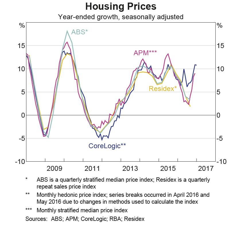
House-and-ArrowRecent developments in Australia have highlighted the fact that there are issues with the metrics here. The RBA has switched from CoreLogic because they suggested this index overstated home price growth, now preferring other index providers. CoreLogic recently discussed their approach.

So the latest IMF working paper – “How to better measure hedonic residential property price indexes” makes interesting reading.

The problem of quality-mix adjustment

Critical to price index measurement is the need to compare, in successive periods, transaction prices of like-with-like representative goods and services. Price index measurement for consumer, producer, and export and import price indexes (CPI, PPI and XMPIs) largely rely on the matched-models method. The detailed specification of one or more representative brand is selected as a high-volume seller in an outlet, for example a single 330 ml. can of regular Coca Cola, and its price recorded. The outlet is then revisited in subsequent months and the price of the self-same item recorded and a geometric average of its price and those of similar such specifications in other outlets form the building blocks of a price index such as the CPI. There may be problems of temporarily missing prices, quality change, say size of can or sold as a bundled part of an offer if bought in bulk, but essentially the price of like is compared with like every month. RPPIs are much harder to measure.

First, there are no transaction prices every month/quarter on the same property. RPPIs have to be compiled from infrequent transactions on heterogeneous properties. A higher (lower) proportion of more expensive houses sold in one quarter should not manifest itself as a measured price increase (decrease). There is a need in measurement to control for changes in the quality of houses sold, a non-trivial task.

The main methods of quality adjustment are (i) hedonic regressions; (ii) use of repeat sales data only; (iii) mix-adjustment by weighting detailed relatively homogeneous strata; and (iv) the sales price appraisal ratio (SPAR). The method selected depends on the database used. There needs to be details of salient price-determining characteristics for hedonic regressions, a relatively large sample of transactions for repeat sales, and good quality appraisal information for SPAR. In the US, for example, price comparisons of repeat sales are mainly used, akin to the like-with-like comparisons of the matched models method, Shiller (1991). There may be bias from not taking full account of depreciation and refurbishment between sales and selectivity bias in only using repeat sales and excluding new home purchases and homes purchased only once. However, the use of repeat sales does not require data on quality characteristics and controls for some immeasurable characteristics that are difficult to effectively include in hedonic regressions, such as a desirable or otherwise view from the property.

The problem of source data

Second, the data sources are generally secondary sources that are not tailor-made by the national statistical offices (NSIs), but collected by third parties, including the land registry/notaries, lenders, realtors (estate agents), and builders. The adequacy of these sources to a large extent depends on a country’s institutional and financial arrangements for purchasing a house and varies between countries in terms of timeliness, coverage (type, vintage, and geographical), price (asking, completion, transaction), method of quality-mix adjustment (repeat sales, hedonic regression, SPAR, square meter) and reliability; pros and cons will vary within and between countries. In the short-medium run users may be dependent on series that have grown up to publicize institutions, such as lenders and realtors, as well as to inform users. Metadata from private organizations may be far from satisfactory.

We stress that our concern here is with measuring RPPIs for FSIs and macroeconomic analysis where the transaction price, that includes structures and land, is of interest. However, for the purpose of national accounts and analysis based thereon, such as productivity, there is a need to both separate the price changes of land from structures and undertake adjustments to price changes due to any quality change on the structures, including depreciation. This is far more complex since separate data on land and structures is not available when a transaction of a property takes place. Diewert, de Haan, and Hendriks (2011) and Diewert and Shimizu (2013a) tackle this difficult problem.

Figure 1 shows alternative data sources in its center and coverage, methods for adjusting for quality mix, nature of the price, and reliability in the four quadrants. Land registry data, for example, may have an excellent coverage of transaction prices, but have relatively few quality characteristics for an effective use of hedonic regressions, not be timely, and have a poor reputation. Lender data may have a biased coverage to certain regions, types of loans, exclude cash sales, have “completion” (of loan) price that may differ from transaction price, but have data on characteristics for hedonic quality adjustment. Realtor data may have good coverage, aside from new houses, data on characteristics for hedonic quality adjustment, but use asking prices rather than transaction prices.

The importance of distinguishing between asking and transaction prices will vary between countries as the length of time between asking and transaction varies with the institutional arrangements for buying and selling a house and the economic cycle of a country.

Whether measurement matters

A natural question is whether the differences in source data and methodologies used matters to the overall outcome of the index. Silver (2015) undertook an extensive formal analysis based on the RPPIs and, as explanatory variables, the associated methodological and source data for 157 RPPIs from 2005:Q1 to 2010:Q1 from 24 countries. The resulting panel data had fixed-time and fixed-country effects; the estimated coefficients on the explanatory measurement variables were first held fixed and then relaxed to be time varying. Subsequently, the explanatory variables were interacted with the country dummies.

imf-indicesThe rest of the paper examines, consolidates, and provides improved practical methods for the timely estimation of hedonic RPPIs, though, as noted earlier, the proposed methods apply equally to CPPIs. Hedonic regressions are the main mechanism recommended for and used by countries for a crucial aspect of RPPI estimation—preventing changes in the quality-mix of properties transacted translating to price changes.

RPPIs and CPPIs are hard to measure. Houses, never mind commercial properties, are infrequently traded and heterogeneous. Average house prices may increase over time, but this may in part be due to a change in the quality-mix of the houses transacted; for example, more 4-bedroom houses in a better (more expensive) post-code transacted in the current period compared with the previous or some distant reference period would bias upwards a measure of change in average prices. A purpose and crucial challenge of RPPIs and CPPIs is to prevent changes in the quality-mix of properties transacted translating to measured price changes. The need is to measure constant-quality property price changes and while there are alternative approaches, the concern of this paper is with the hedonic approach as a recommended widely used methodology for this.


Note: IMF Working Papers describe research in progress by the author(s) and are published to elicit comments and to encourage debate. The views expressed in IMF Working Papers are those of the author(s) and do not necessarily represent the views of the IMF, its Executive Board, or IMF management.

The Deadly Grip Of Property Depression In The Mining Belt

Important analysis from CoreLogic showing the impact of the property downturn on the mining belt.

As commodity prices and mining investment has sunk, demand for housing in mining areas has also slowed. This week we take a look at the performance of some of the major mining towns.

Mining towns and regions across the country have been hard hit as investment and commodity prices have slumped.  This week we’re looking at how the housing market has performed in terms of the volume and median price of sales across these regions.  The results indicate that not all mining towns have recorded an equivalent slowdown.  The following analysis looks at annual median prices and annual sales volumes

Port Hedland – median prices peaked at $925,000 in June 2013 and sales volumes peaked at 402 in July 2006.  Current median prices are $390,000 (-58% lower than peak) and current sales are 128 (-68% below peak).  In what may be a positive sign for the market, annual sales are once again trending higher, although the median prices trend is yet to bottom out.

2016-11-07--image1

Isaac – median prices peaked at $620,000 in November 2012 and sales volumes peaked at 661 in March 2012.  Current median prices are $138,390 (-78% lower than peak) and current sales are 117 (-28% below peak).  Transaction numbers have recently started to rise, however median price trends remain negative.

2016-11-07--image2

Karratha – median prices peaked at $815,000 in October 2010 and sales volumes peaked at 511 in March 2005.  Current median prices are $362,980 (-55% lower than peak) and current sales are 235 (-54% below peak).  Transaction numbers have been trending higher since xxx but the median sale price is still falling, albeit at a more moderate pace.

2016-11-07--image3

Gladstone – median prices peaked at $475,000 in September 2012 and sales volumes peaked at 1,823 in July 2007.  Current median prices are $350,000 (-26% lower than peak) and current sales are 572 (-69% below peak).  Dwelling turnover is continuing along a downwards trend with no sign of an improvement in buyer demand just yet.

2016-11-07--image4

Kalgoorlie-Boulder – median prices peaked at $351,250 in June 2015 and sales volumes peaked at 1,656 in September 2006.  Current median prices are $312,000 (-11% lower than peak) and current sales are 345 (-79% below peak).  Transaction numbers appear to be levelling, however there is no sign of any upwards pressure on prices or turnover.

2016-11-07--image5

Mackay – median prices peaked at $435,000 in June 2013 and sales volumes peaked at 3,264 in April 2004.  Current median prices are $345,000 (-21% lower than peak) and current sales are 1,045 (-68% below peak).  Transaction numbers have recently levelled across the Mackay housing market but are yet to improve.

2016-07-11--image6

Roxby Downs – median prices peaked at $500,016 in November 2013 and sales volumes peaked at 187 in February 2004.  Current median prices are $250,000 (-50% lower than peak) and current sales are 23 (-88% below peak).  Transaction numbers have recently increased slightly across Roxby Downs.

2016-11-07--image7

The smaller mining townships which don’t act as major service centres have tended to see a much sharper fall in median selling prices than the larger townships.  The decline in sales and prices from the market peaks has been substantial across all of these regions, however the regions that have seen the most significant downturn were those that also recorded a significant upswing in prices and turnover rates prior to the peak in commodity prices.

Recently, most of these mining towns have experienced a stabilisation in sales with some regions having seen an increase in sales volumes.  Although sales may have broken the declining trend in a number of areas, median selling prices are generally continuing to trend lower across each of the regions highlighted. The improvement in transactional activity could potentially be due to larger numbers of distressed sales moving through these markets, but may also be attributable to a cautious return of buyers seeking out a bargain.

The challenge for many of these regions remains that despite a recent uptick in commodity prices, investment in large infrastructure projects (new mines, processing facilities, transport etc) has dried up and subsequently few additional jobs are being created.  Although commodity prices have recently surged, particular iron ore, coking coal and thermal coal, it is not yet leading to a substantial increase in exploration activity or employment, subsequently housing demand remains weak and continues to have a dampening effect on housing prices.

RBA Still Sanguine On Housing

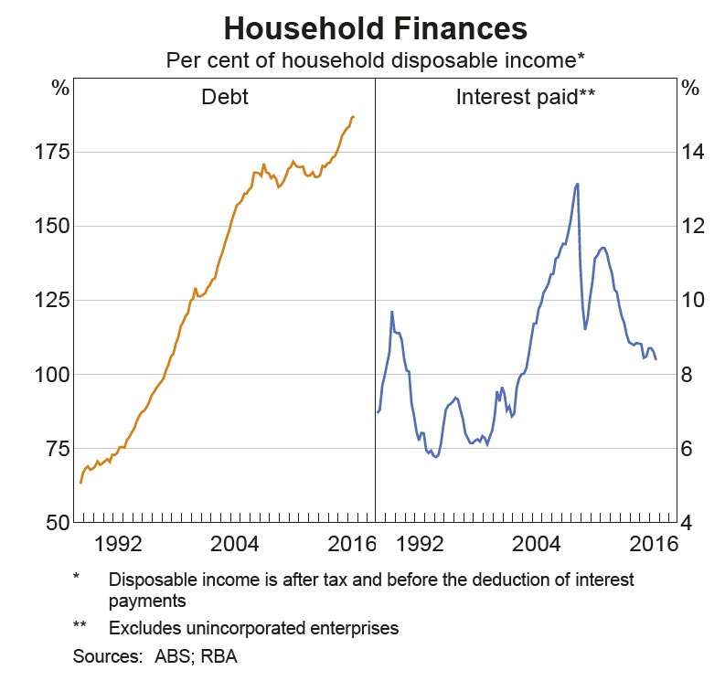
The latest RBA Statement of Monetary Policy, released today includes a range of comments on housing, and mortgage lending. Clearly the RBA wants to continue to show there is nothing to see here. High absolute household debt and rising defaults hardly gets a mention! They also choose to use the APM home price data rather than CoreLogic’s indices (which would show higher growth). They say the average outstanding housing interest rate has fallen by around 35 basis points this year.

However, they do warn that if growth in housing demand does not continue to keep pace with the scheduled large increases in supply, it would place downward pressure on housing prices and rents and increase the risk of off-the-plan apartment purchases failing to settle.

They also warn that if the broader housing market was to weaken substantially, consumption growth may be lower than currently expected in response to wealth and income effects. Consumer price inflation would also be affected as housing costs comprise a significant share of household expenditure.

rba-housing-nov-2016As expected, private dwelling investment was strong over the year to the June quarter. The value of residential building approvals has reached record levels as a share of GDP and the amount of work in the pipeline has edged higher. Accordingly, dwelling investment is likely to contribute to growth for some time yet. However, the large amount of work in the pipeline raises concerns that some locations could become oversupplied, particularly in inner-city areas where a lot of highdensity housing is planned. This could lead to settlement failures by off-the-plan purchasers and a general reduction in rents and prices.

rba-nov-16-house-prices Conditions in the established housing market have eased relative to a year ago, although some indicators suggest that conditions may have strengthened over recent months. In particular, housing price growth has picked up noticeably in Sydney and Melbourne, where auction clearance rates have also increased to high levels.

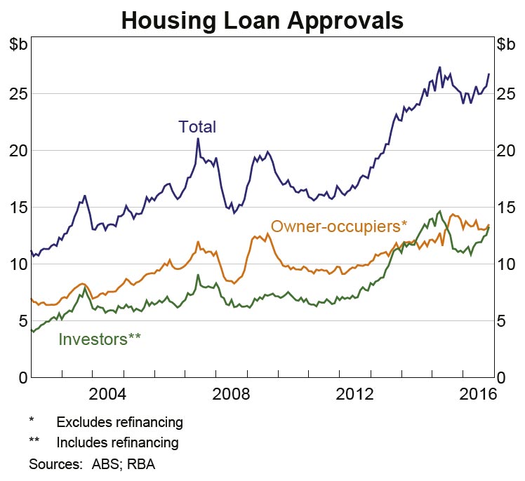
rba-nov16-housing-indHowever, the number of auctions and housing market turnover more generally are lower than they were last year and  properties are, on average, taking longer to sell. While housing credit growth has also declined over the past year, loan approvals data suggest that lending to investors has increased a little over recent months. Housing market conditions remain weak in Perth, where prices of both apartments and detached dwellings have declined further over the past year.

rba-nov16-rentalsHousing credit growth has eased to an annualised pace of around 6 per cent. Growth in net housing debt is about 1 percentage point below growth in housing credit due to ongoing strong growth in deposits in mortgage offset accounts.

While the slowing in housing credit growth and loan approvals has been reasonably broad based, there remains some divergence in the pace of growth across states (Graph 4.11). The slowing in loan approvals has been particularly pronounced in Western Australia; while loan approvals in NSW have also eased over the past year, they continue at a pace noticeably above the national average.

rba-nov16-lendingGrowth in credit advanced to investors has increased a little in recent months, consistent with a pick-up in investor housing loan approvals. In contrast, growth in credit advanced to owner-occupiers has eased a little recently. The current level of approvals is consistent with housing credit growth continuing at around its current pace.

The slowing in housing loan approvals over the past year is consistent with the decline in turnover in the housing market. It also reflects slower growth in average dwelling prices and a decrease in the average loan-to-valuation ratio. The latter follows the introduction of measures by the Australian Prudential Regulation Authority (APRA) to strengthen lending standards. Another factor that  may be contributing to the easing in housing credit growth over the past year is an increase in the share of off-the-plan purchases, which are yet to flow through to the demand for credit. These transactions do not involve a mortgage at the time the dwelling is purchased off the plan, but add to the stock of housing credit when a mortgage is provided to the purchaser upon completion of the dwelling.

Around half of the August cash rate reduction was passed through to most advertised housing lending rates. The average outstanding housing interest rate has fallen by around 35 basis points this year and is likely to decline a little further as maturing loans are replaced with loans on lower The lowest available variable interest rates are more than 50 basis points below the average outstanding interest rate and, reflecting the lower rates on offer, the level of refinancing activity remains relatively high. One bank has recently introduced a loan product with the interest rate margin fixed at 249 basis points above the cash rate.

Recent strength in dwelling investment, particularly the construction of higher-density dwellings, has played a role in supporting the rebalancing of economic activity away from the resources sector.

Low interest rates and increases in housing prices have encouraged a substantial increase in the supply of apartments and the pipeline of residential work yet to be done has increased to historically high levels. While this pipeline should support growth in dwelling investment over the next year or so, the outlook for dwelling investment beyond this period is uncertain.

There is concern about the risk of an oversupply of apartments in specific geographical areas, such as inner-city areas of Melbourne and Brisbane. Outside Western Australia, the supply of housing has to date largely been absorbed by population growth. However, if growth in housing demand does not continue to keep pace with the scheduled large increases in supply, it would place downward pressure on housing prices and rents and increase the risk of off-the-plan apartment purchases failing to settle. If the broader housing market was to weaken substantially, consumption growth may be lower than currently expected in response to wealth and income effects. Consumer price inflation would also be affected as housing costs comprise a significant share of household expenditure.

A Recipe To Tackle Housing Affordability

KPMG has released a brief report “Housing Affordability: What can be done about the Great Australian Dream? They exhibit greater joined up thinking than recent Government outings, because they include tax reform, supply of affordable housing and shared equity options as part of a reform package. It also shows how complex the issues are.  They say it should be a focus of public policy.

The missing piece of the puzzle though for me is property price sentiment. In a rising market, expectations of future price rises drive prices higher, and when two thirds of voters have direct interests in property and the wealth effect these price rises create, it would be a courageous politician who rocks the “magic pudding” boat! Rather they will tinker ineffectively at the margins.

There is no doubt that Australia is experiencing a worsening problem regarding housing affordability, a fact highlighted this week (24 October 2016) by the Federal Treasurer in a speech to the Urban Development Institute of Australia.

kpmgThe driver of reduced affordability has clearly been the rapid increase in the price of housing, relative to a more benign adjustment in household incomes.

Many of the drivers of house price increases and affordability pressures on some households are occurring globally, are largely macroeconomic and are the product of a complex interaction of demand and supply side factors, and no single policy intervention will address the entire issue.

About a decade ago KPMG Economics completed a detailed review into housing affordability in Australia. At the time we found that the change in median house prices were mostly influenced by the underlying strength of the economy, the performance of the share market, and the proportion of housing being purchased by investors relative to owner occupiers.

We have just re-investigated the relationship of median housing prices in Australia to the key drivers identified a decade ago and found GDP and investor activity remain key influences, but the share market no longer had such an influential role. However, wages, interest rates and housing supply are factors whose influence on house prices have strengthened over the past decade.

Average access to intergenerational equity – being the average amount of time a generation has access to potential wealth via inheritance from the immediately preceding generation – is anticipated to be greatest for ‘Baby Boomers’, and least for ‘Generation X’.

We are now seeing a change in behavior by current generations regarding home purchasing which is new compared to previous generations. That is, some young people are now collaborating to buy, some are assisted by parents, while others are simply choosing not to buy because they don’t want to be committed to a location for 30 years of a mortgage.

Low income households are only able to afford housing stock that is located on the fringe of cities, and even then this has become more difficult. However, this outwards push of the urban fringe also creates broader issues for society around provision of infrastructure into these ‘greenfield locations’, and the false economies associated with cheaper housing but more expensive private and public transport.

KPMG recognises the challenges associated with resolving the problem of housing affordability are complex and they involve a range of both supply and demand side factors. We have offered a number of solutions that provide a way forward for housing affordability to be improved on a permanent basis.

These include:

1. CGT reduction: reducing the capital gains tax discount from 50% to 25%, thereby making property investment marginally less attractive
2. Aggregate property tax: abolish stamp duty on the transfer of residential property and conflate rates, land tax, insurance taxes and emergency service levies into a new Property Services Tax
3. Systemic reforms aimed at maintaining the supply and diversity of land and housing in established and growth areas, through:
a) Set targets: a stronger role for target setting for “net additions to stock” to drive Local and State Government planning schemes;
b) Affordable product: target setting would also focus on encouraging greater diversity of housing stock and deliberately encouraging smaller, well designed affordable products;
c) Streamline planning: making further improvements to the planning system to capitalise on the Government’s planned use of structure plans as a means of reducing the holding costs associated with planning delays – and providing developers in both the private and public sector with greater capacity and incentives to bolster supply at times when the market is under substantial demand pressure;
d) Empower public supply: supporting a stronger role for government land authorities to focus on housing affordability for middle income households within the context of a broader sustainability agenda.
4. Targeted Reforms aimed at improving access to those groups who are the most excluded from affordable home ownership. This package would focus on:
a) More low cost housing: the production of a greater volume of more sustainable, well-designed, lower cost house and land packages;
b) Improve assistance: better targeting of existing State first home owner assistance to increase the overall value and impact of that assistance;
c) Promote shared equity: the introduction of a shared equity program with a percentage of that equity exempt from rental interest charges for the life of the loan or a part of it to be provided by Government and/or the private sector.

KPMG also believes that the solution for Australia must involve all levels of Government working together, given the factors driving the problems are not under the remit of any one level of government. It should be a priority area of public policy.

Home Prices Higher In Most States – CoreLogic

CoreLogic says that capital city dwelling values shift half a percent higher in October 2016 based on their Home Value Index. They have reached a new record high for the month, with values rising across six of the eight capitals.

Apart from Adelaide (-1.3%), Hobart (-2.8%) and Perth (-1.5%), every capital city recorded a rise in dwelling values over the past three months, with the Canberra housing market recording the largest increase in values after a 5.6% quarterly rise.

corelogic-october-2016-1Sydney continued as the stand out based on annual capital gains, recording the largest year-on-year increase; dwelling values are now 10.6% higher over the past 12 months. Detached houses (+10.9%) are showing only a slightly higher rate of capital gain compared with units (+9.1%) across Sydney, highlighting the healthier supply/demand dynamic that exists across the Sydney region for higher density housing.

The divergence in performance between houses and units is most clearly evident in Melbourne and Brisbane. The annual rate of capital gains in Melbourne remains strong at 9.1%, however there is a substantial difference in growth rates between houses and units, with house values up 9.6% compared with a 5.2% increase in unit values over the past year. Brisbane’s housing market has shown a larger capital gain spread, with house values up 4.7% compared with a 1.4% fall in unit values over the year.

According to CoreLogic, another sign of market strength can be seen in auction results. In fact, over the past two months, clearance rates across Sydney have dipped below 80% only once. A year ago auction clearance rates were consistently trending around the mid 60% range, albeit on volumes that were about 20% lower than last year.

While dwelling values have broadly risen during October, rental yields in Sydney and Melbourne remain depressed, with gross yields at record lows. The typical Sydney and Melbourne house is now providing a gross rental return of just 2.8%. Taking into consideration holdings costs, expenses and vacancy, the net rental yield for houses is likely to be closer to 2% in these markets. Markets where value growth hasn’t been as strong are seeing healthier yield profiles, with Hobart demonstrating the highest gross rental yields of any capital city.

corelogic-october-2016-2