Federal Reserve – Page 31 – Digital Finance Analytics (DFA) Blog

Fed Holds Rates Once Again

Whilst the Fed highlighted some further improvements in the US economy, and three board members wanted to lift, the decision was to hold. The markets liked the decision, reflecting on the fact that with the November Fed meeting abutting the US election, December is the likely next window.

Information received since the Federal Open Market Committee met in July indicates that the labor market has continued to strengthen and growth of economic activity has picked up from the modest pace seen in the first half of this year. Although the unemployment rate is little changed in recent months, job gains have been solid, on average. Household spending has been growing strongly but business fixed investment has remained soft. Inflation has continued to run below the Committee’s 2 percent longer-run objective, partly reflecting earlier declines in energy prices and in prices of non-energy imports. Market-based measures of inflation compensation remain low; most survey-based measures of longer-term inflation expectations are little changed, on balance, in recent months.

Consistent with its statutory mandate, the Committee seeks to foster maximum employment and price stability. The Committee expects that, with gradual adjustments in the stance of monetary policy, economic activity will expand at a moderate pace and labor market conditions will strengthen somewhat further. Inflation is expected to remain low in the near term, in part because of earlier declines in energy prices, but to rise to 2 percent over the medium term as the transitory effects of past declines in energy and import prices dissipate and the labor market strengthens further. Near-term risks to the economic outlook appear roughly balanced. The Committee continues to closely monitor inflation indicators and global economic and financial developments.

Against this backdrop, the Committee decided to maintain the target range for the federal funds rate at 1/4 to 1/2 percent. The Committee judges that the case for an increase in the federal funds rate has strengthened but decided, for the time being, to wait for further evidence of continued progress toward its objectives. The stance of monetary policy remains accommodative, thereby supporting further improvement in labor market conditions and a return to 2 percent inflation.

In determining the timing and size of future adjustments to the target range for the federal funds rate, the Committee will assess realized and expected economic conditions relative to its objectives of maximum employment and 2 percent inflation. This assessment will take into account a wide range of information, including measures of labor market conditions, indicators of inflation pressures and inflation expectations, and readings on financial and international developments. In light of the current shortfall of inflation from 2 percent, the Committee will carefully monitor actual and expected progress toward its inflation goal. The Committee expects that economic conditions will evolve in a manner that will warrant only gradual increases in the federal funds rate; the federal funds rate is likely to remain, for some time, below levels that are expected to prevail in the longer run. However, the actual path of the federal funds rate will depend on the economic outlook as informed by incoming data.

The Committee is maintaining its existing policy of reinvesting principal payments from its holdings of agency debt and agency mortgage-backed securities in agency mortgage-backed securities and of rolling over maturing Treasury securities at auction, and it anticipates doing so until normalization of the level of the federal funds rate is well under way. This policy, by keeping the Committee’s holdings of longer-term securities at sizable levels, should help maintain accommodative financial conditions.

Voting for the FOMC monetary policy action were: Janet L. Yellen, Chair; William C. Dudley, Vice Chairman; Lael Brainard; James Bullard; Stanley Fischer; Jerome H. Powell; and Daniel K. Tarullo. Voting against the action were: Esther L. George, Loretta J. Mester, and Eric Rosengren, each of whom preferred at this meeting to raise the target range for the federal funds rate to 1/2 to 3/4 percent.

US Household Net Worth Rises

The latest (Q2 16) US Financial Accounts have been released, containing data on the flow of funds and levels of financial assets and liabilities. The data will increase the likelihood of a fed rate rise, offsetting the more negative news released yesterday.

The net worth of households and nonprofits rose to $89.1 trillion during the second quarter of 2016. The value of directly and indirectly held corporate equities increased $452 billion and the value of real estate rose $474 billion. The figure plots the contributions to the change in net worth of households and nonprofit organizations. The black line plots the total change in net worth, while the bars represent the changes in the main components of net worth: market value of directly and indirectly held corporate equity (dark blue), market value of real estate holdings (green), and other assets net of liabilities (light blue). Other assets include consumer durable goods, nonprofit organizations’ fixed assets, and financial assets other than corporate equity.

Household debt increased at an annual rate of 4.4 percent in the second quarter of 2016. Consumer credit grew 6.4 percent, while mortgage debt (excluding charge-offs) grew 2.5 percent at an annual rate.

Domestic nonfinancial debt outstanding was $46.3 trillion at the end of the second quarter of 2016, of which household debt was $14.5 trillion, nonfinancial business debt was $13.2 trillion, and total government debt was $18.6 trillion. The figure plots the 4-quarter moving average percent growth rate of debt outstanding for domestic nonfinancial sectors at a quarterly frequency. The growth rate of debt is calculated as the seasonally adjusted flow divided by the seasonally adjusted level in the previous period, multiplied by 100. In the Financial Accounts, debt equals the sum of debt securities and loans.

Domestic nonfinancial debt growth was 4.4 percent at a seasonally adjusted annual rate in the second quarter of 2016, down from an annual rate of 5.4 percent in the previous quarter.

Nonfinancial business debt rose at an annual rate of 4.1 percent in the second quarter, down from an annual rate of 9.4 percent in the previous quarter.

State and local government debt rose at an annual rate of 2.2 percent in the second quarter of 2016, up from an annual growth rate of 0.8 percent in the previous quarter.

Federal government debt increased 5.0 percent at a seasonally adjusted annual rate in the second quarter of 2016.

Rate Hikes Will Be the Least of Market Worries – Moody’s

Moody’s says the Fed does not set interest rates in a vacuum. Indeed, the federal funds rate is shaped by a host of drivers that are hardly limited to labor market conditions.

Despite warnings from high-ranking Fed officials that ultra-low interest rates are not forever, recent soundings of business activity, as well as the nearness of November 8’s Presidential election, weigh against a hiking of the federal funds rate prior to the FOMC’s December 14 meeting. Moreover, recent data question whether 2016 will be home to even a single rate hike.

In a September 12 speech, Fed governor Lael Brainard presented a convincing case favoring an extended stay by exceptionally low benchmark interest rates. On several occasions, Governor Brainard challenged the wisdom of a preemptive rate hike that intends to thwart inflation before it takes hold. Given “the absence of accelerating inflationary pressures” and the limited scope for lowering of fed funds in the event recession risks rise, Brainard argues for the continuation of a highly accommodative monetary policy. Basically, the macroeconomic costs of mistakenly hiking rates too early are viewed as well exceeding the potential inflationary costs of waiting too long to confront inflation. The damage done by a premature rate hike may be harder to repair than the damage resulting from above-target price inflation.

However, there is an alternative view that views ultra-low interest rates as doing more harm than good because of how cheap money (i) boosts savings in order to compensate for negligible interest income and (ii) forces investors to purchase riskier assets offering higher, though volatile, returns.

Futures now sense 2016 will end without a rate hike

As measured by the CME Group’s FedWatch tool, fed funds futures assign an implied probability of only 12% to a hiking of fed funds at the September 21 meeting of the FOMC. Thereafter, the implied likelihood barely rises to 20% for the November 2 meeting and climbs no higher than 47% for the FOMC’s deliberations of December 14. For now, the futures market does not expect a single rate hike for 2016.

The latest declines by the implied probabilities of rate hikes at the FOMC’s remaining three meetings for 2016 stemmed from lower than expected August readings for retail sales and industrial production. Despite the latest indications of subpar business sales, US equities rallied. Moreover, an accompanying drop by the VIX index hinted a narrowing of the high-yield spread that recently widened from September 8’s 18-month low of 508 bp to September 14’s 538 bp. Nevertheless, at some point, the corporate earnings outlook will overrule the now predominant influence of Fed policy. Unless business sales soon accelerate sufficiently, market participants will begin to fret over the adequacy of earnings for 2016’s final quarter and all of 2017.

US Production Index Lower Than Expected

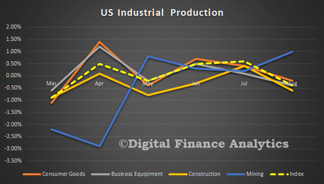
Latest figures from the US Federal Reserve shows that industrial production decreased 0.4 percent in August after rising 0.6 percent in July. The market reacted to this data, taking it as an indicator that a rate rise was less likely in the short term.

Manufacturing output declined 0.4 percent in August, reversing its increase in July; the level of the index in August is little changed from its level in March. Following two consecutive monthly increases, the index for utilities fell back 1.4 percent in August. Even so, the index was 1.7 percent above its year-earlier level, as hot temperatures this summer boosted the usage of air conditioning.

The output of mining moved up 1.0 percent in August, its fourth consecutive monthly increase following an extended downturn; the index, however, was still about 9 percent below its year-ago level. At 104.4 percent of its 2012 average, total industrial production in August was 1.1 percent lower than its year-earlier level. Capacity utilization for the industrial sector decreased 0.4 percentage point in August to 75.5 percent, a rate that is 4.5 percentage points below its long-run (1972–2015) average.

Market Groups

The indexes for all major market groups declined in August. The output of consumer goods decreased 0.2 percent as a result of a large drop in consumer energy products and a small decline in consumer non-energy nondurables. The output of consumer durables was unchanged; a gain in automotive products was offset by declines in all of its other components. Business equipment posted a decrease of 0.4 percent, as gains of 1 percent or more for transit equipment and for information processing equipment were outweighed by a cutback of nearly 2 percent for industrial and other equipment. The output of defense and space equipment declined 0.6 percent. The indexes for construction supplies and business supplies moved down 0.6 percent and 0.8 percent, respectively. The production of materials decreased 0.5 percent: Both durable and energy materials posted declines, while the output of nondurable materials was unchanged. The reduction in the index for durable materials reflected similarly sized losses across all its major categories.

Industry Groups

Manufacturing output declined 0.4 percent in August; the index was also 0.4 percent below its level of a year earlier. In August, the production of nondurables moved down 0.2 percent, and the indexes for durables and for other manufacturing (publishing and logging) fell 0.6 percent and 0.7 percent, respectively. Many durable goods industries posted declines of nearly 1 percent or more, with the largest drop, 1.9 percent, recorded by machinery. Within nondurables, gains for food, beverage, and tobacco products and for paper were more than offset by declines elsewhere; the largest decrease, 2.1 percent, was recorded by textile and product mills.

The index for mining moved up 1.0 percent in August, with a decline in coal mining outweighed by increases in the indexes for oil and gas extraction, for oil well drilling and servicing, and for metal ore and nonmetallic mineral mining.

Capacity utilization for manufacturing decreased 0.4 percentage point in August to 74.8 percent, a rate that is 3.7 percentage points below its long-run average. The operating rate for nondurables moved down 0.2 percentage point; the rates for durables and for other manufacturing (publishing and logging) each declined 0.5 percentage point. The operating rate for mining moved up 1.0 percentage point to 76.2 percent, while the rate for utilities decreased 1.3 percentage points to 80.4 percent.

The “New Normal” and US Rates

Recent volatile stock market movements are in reaction to the fear that central banks will begin to tighten monetary policy. Much attention is on the Federal Reserve. So, a significant speech from Fed Governor Lael Brainard is worth noting. She spoke at the Chicago Council on Global Affairs, Chicago, Illinois and outlined five factors in “the new normal”.

She concludes:

The five features of the current economic landscape that I have highlighted lean roughly in the same direction: In today’s new normal, the costs to the economy of greater-than-expected strength in demand are likely to be lower than the costs of significant unexpected weakness. In the case of unexpected strength, we have well-tried and tested tools and ample policy space in which to react. Moreover, because of Phillips curve flattening, the possibility of remaining labor market slack, the likely substantial response of the exchange rate and its depressing effect on inflation, the low neutral rate, and the fact that inflation expectations are well anchored to the upside, the response of inflation to unexpected strength in demand will likely be modest and gradual, requiring a correspondingly moderate policy response and implying relatively slight costs to the economy. In the face of an adverse shock, however, our conventional policy toolkit is more limited, and thus the risk of being unable to adequately respond to unexpected weakness is greater. The experience of the Japanese and euro-area economies suggest that prolonged weakness in demand is very difficult to correct, leading to economic costs that can be considerable.

This asymmetry in risk management in today’s new normal counsels prudence in the removal of policy accommodation. I believe this approach has served us well in recent months, helping to support continued gains in employment and progress on inflation. I look forward to assessing the evolution of the data in the months ahead for signs of further progress toward our goals, bearing in mind these considerations.

Watch her speech in full.

1. Inflation Has Been Undershooting, and the Phillips Curve Has Flattened
First, for the past several decades, policymakers relied on the empirical relationship between unemployment and inflation embodied in the Phillips curve as a key guidepost for monetary policy. The Phillips curve implied that as labor market slack diminished and the economy approached full employment, upward pressure on inflation would result. However, since 2012, inflation has tended to change relatively little–both absolutely and relative to earlier decades–as the unemployment rate has fallen considerably. At a time when the unemployment rate has fallen from 8.2 percent to 4.9 percent, inflation has undershot our 2 percent target now for 51 straight months. In other words, the Phillips curve appears to be flatter today than it was previously.

2. Labor Market Slack Has Been Greater than Anticipated
Second, and related, although we have seen important progress on employment, this improvement has been accompanied by evidence of greater slack than previously anticipated. This uncertainty about the true state of the economy suggests we should be open to the possibility of material further progress in the labor market. Indeed, with payroll employment growth averaging 180,000 per month this year, many observers would have expected the unemployment rate to drop noticeably rather than moving sideways, as it has done. It is true that today’s unemployment rate of 4.9 percent is only 0.1 percentage point from the median SEP participant’s estimate of the longer-run level of unemployment. However, the natural rate of unemployment is uncertain and can vary over time. Indeed, in the SEP, the central tendency of the projection for the longer-run natural rate of unemployment has come down significantly, from a range of 5.2 to 6.0 percent in June 2012 to 4.7 to 5.0 percent in June 2016–a reduction of 1/2 to 1 percentage point. We cannot rule out that estimates of the natural unemployment rate may move even lower.

3. Foreign Markets Matter, Especially because Financial Transmission is Strong
Third, disinflation pressure and weak demand from abroad will likely weigh on the U.S. outlook for some time, and fragility in global markets could again pose risks here at home. In Europe, recovery continues, but growth is slow and inflation is very low. Low growth and a flat yield curve are contributing to reduced profitability and a higher cost of equity financing for banks, which in turn could impair bank lending, one of the main transmission channels of monetary policy in the euro area’s bank-centric financial system. A low growth, low inflation environment also makes progress on fiscal sustainability difficult and leaves countries with high debt-to-gross domestic product (GDP) ratios vulnerable to adverse demand shocks. Against this backdrop, uncertainty about Britain’s future relationship with the European Union could damp business sentiment and investment in Europe.

4. The Neutral Rate Is Likely to Remain Very Low for Some Time
Fourth, perhaps most salient for monetary policy, it appears increasingly clear that the neutral rate of interest remains considerably and persistently lower than it was before the crisis. Over the current expansion, with a federal funds rate at, or near, zero and the additional support provided by asset purchases and reinvestment, GDP growth has averaged a very modest rate upward of 2 percent, and inflation has averaged only 1‑1/2 percent. Ten years ago, based on the underlying economic relationships that prevailed at the time, it would have seemed inconceivable that real activity and inflation would be so subdued given the stance of monetary policy. To reconcile these developments, it is difficult not to conclude that the current level of the federal funds rate is less accommodative today than it would have been 10 years ago. Put differently, the amount of aggregate demand associated with a given level of the interest rate is now much lower than before the crisis.

5. Policy Options Are Asymmetric
The four features just discussed that define the new normal make it likely that we will continue to grapple with a fifth new reality for some time: the ability of monetary policy to respond to shocks is asymmetric. With policy rates near the zero lower bound and likely to return there more frequently even if the economy only experiences shocks similar in magnitude to those experienced pre-crisis, due to the low level of the neutral rate, there is an asymmetry in the policy tools available to respond to adverse developments. Conventional changes in the federal funds rate, our most tested and best understood tool, cannot be used as readily to respond to downside shocks to aggregate demand as it can to upside shocks. While there are, of course, other policy options, these alternatives have constraints and uncertainties that are not present with conventional policy. From a risk-management perspective, therefore, the asymmetry in the conventional policy toolkit would lead me to expect policy to be tilted somewhat in favor of guarding against downside risks relative to preemptively raising rates to guard against upside risks.

Long-Run Economic Effects of Changes in the Age Dependency Ratio

A decrease in the labor force and an increase in the elderly population could slow economic growth, says economic research from the Federal Reserve Bank of St. Louis.

Important demographic changes in the developed world in recent years may have long-run economic consequences. As a result, such changes have started to play a more important role in the design of economic policies.

In a recent blog post, I analyzed changes in the age dependency ratio in the G-7 countries since 1990.¹ Thorough analysis of the evolution of this variable and its components is important because the young and old are likely to be more economically dependent on the rest of the population and changes in age composition may affect other areas of the economy.

Panel A of the figure plots the annual age dependency ratios for the G-7 countries from 1990 to 2012. The age dependency ratio is the sum of the young population (under age 15) and elderly population (age 65 and over) relative to the working-age population (ages 15 to 64). As the figure shows, dependency ratios have risen in all seven countries in the past 10 years. In some countries, however, the trend started earlier. In Japan, for instance, the increase started in the early 1990s. Changes in the age composition of the population—from increases and/or decreases in the young and elderly populations—drive the dependency ratios. As the figure shows, in all G-7 countries, the elderly populations (Panel B) have increased, while the working-age populations (Panel C) and young populations (Panel D) have decreased slightly or stayed flat. Among those countries, Japan’s age dependency ratio increased the most.

Several recent studies² suggest that high dependency ratios may have the following long-term economic
consequences:

Saving rates: As workers get close to retirement, they tend to increase their savings through pension plans, healthcare insurance, etc. Also, if younger workers anticipate changes in demographic trends, they could start saving more for the future (by investing more in private pension plans, postponing consumption decisions, or investing in private health insurance). Increased savings could have long-term economic consequences, such as a decrease in long-term interest rates. Eventually, as the elderly start retiring and birth rates start decreasing—as appears to be the recent trend—savings would start decreasing and long-term interest rates would rise. Thus, recent demographic changes could affect saving rates and long-term interest rates.

Investment rates: If savings decrease, there could be fewer funds to finance investment projects, which could decrease investment in physical capital. Decreased investment could reduce long-term economic growth.

Housing markets: A growing labor force would increase house prices. A recent article in The Economist finds that since 1960, house prices in a sample of 10 countries fell by 0.2 percent per year as the age dependency ratio increased. Because the demographic composition of the labor force contributes strongly to the trend in house prices, fewer young people, together with a large increase in the elderly population, would likely result in less investment in the housing market.

Consumption patterns: An increase in the elderly population could shift consumption from certain goods toward healthcare services and leisure.

In summary, the decrease in the labor force, due to an increase in the elderly population and a decrease in the fertility rate, could translate into lower economic growth. Long-term problems in the developed world caused by an increase in the age dependency ratio could be alleviated by either increasing productivity (to avoid an economic slow-down from a shrinking labor force) or increasing the labor force participation of the elderly (e.g., by increasing the retirement age, as several European countries have done recently, or reducing taxes on the labor income of elderly workers). These economic policies, however, would not reverse the recent demographic trends.

Notes

¹ Santacreu, Ana Maria. “How Are Populations Shifting within Developed Countries?” Federal Reserve Bank of St. Louis On The Economy Blog, August 11, 2016; https://www.stlouisfed.org/on-the-economy/2016/aug….

² Economist. “Vanishing Workers.” July 2016, 420(8999), p. 58, http://www.economist.com/news/finance-and-economic…. Karp, Nathaniel and Nash-Stacey, Boyd. “Slow Productivity Growth: Cracking the Code.” BBVA Research U.S. Economic Watch, August 4, 2016; https://www.bbvaresearch.com/wp-content/uploads/20….

The Timing of Labeling a Bank “Too Big to Fail” Matters

From the St. Louis Fed On The Economy Blog.

When banks that are considered “too big to fail” (TBTF) are on the verge of failure and are subsequently saved by the government, many argue that the government is bailing out stock and bond holders at taxpayer expense. However, exactly who gets bailed out may be unclear. An Economic Synopses essay argues that it depends on when the institution is labeled TBTF.

Director of Research Christopher Waller noted that current stock and bond holders of failing banks get bailed out if the institutions are unexpectedly declared TBTF at the moment they are about to default. This is because markets haven’t had time to incorporate the TBTF news into asset prices.

However, it’s when banks are considered TBTF prior to default that the issue of who gets bailed out becomes murkier. Waller quoted authors of a 2004 book Ron Feldman and Gary Stern about the problem: “‘The roots of the TBTF problem lie in creditors’ expectations … and the source of the problem is a lack of credibility’ that the government will let them fail.”¹ Waller wrote: “It is exactly this timing that makes it difficult to determine who benefits from TBTF.”

A TBTF Announcement and Reaction

Waller gave an example of a bank (which he simply called bank A) that had been declared TBTF by the government. In response, the prices of the bank’s stocks and bonds would rise to reflect this new information. Subsequent offerings would also have higher prices, again due to the TBTF designation (and corresponding lack of default risk).

Investors who buy this bank’s stocks or bonds after the announcement, however, wouldn’t necessarily see a benefit. Waller noted that the TBTF status should be fully incorporated into asset prices, assuming financial markets are efficient. He wrote: “In short, new buyers are paying for the TBTF insurance via higher equity and bond prices. They do not receive a windfall from the TBTF status assigned to bank A.”

What If the Bank Is Allowed to Fail?

Waller also addressed what would happen if the bank was still allowed to fail after the TBTF designation was given. He wrote that initial bond and stock holders who sold after the announcement would not care, as they already received the insurance premium and would not be affected by the failure.

The current holders, however, would have paid a premium for the insurance, only to lose their investments anyway. Waller wrote: “Hence, it is not surprising that they would be upset by the government’s action. Who wouldn’t be upset after paying for insurance that didn’t pay off when it should have?”

Conclusion

Waller wrote: “To summarize, the value of being designated TBTF is capitalized into the price of a firm’s equities and its bonds. TBTF provides a windfall capital gain to shareholders and creditors at the time of the designation. But after that, new buyers of equities and debt are paying for that status. Consequently, determining who gets ‘bailed out’ when an institution is TBTF is a more complicated task than it appears.”

Notes and References

¹ Feldman, Ron; and Stern, Gary. Too Big to Fail: The Hazards of Bank Bailouts. Washington, D.C.: Brookings Institution Press, 2004.

Fed Leaves September Rate Hike Option Live

Monetary policy is alive and well, according to the FED, and interest rate rises are on the cards in the US. Chair Janet L. Yellen spoke at “Designing Resilient Monetary Policy Frameworks for the Future,” a symposium sponsored by the Federal Reserve Bank of Kansas City, Jackson Hole, Wyoming, her speech was entitled “The Federal Reserve’s Monetary Policy Toolkit: Past, Present, and Future.”

The AU/US dollar moved in reaction to the speech.

In a nutshell, monetary policy remains relevant, and given the current economic indicators, there appears scope for rate rises later this year, possibly as soon as September. Her comments on how rate adjustments have been simulated are worth reading. It also means that we may see some falls in asset prices as the rises bite, across stocks and property.

A recent paper takes a different approach to assessing the FOMC’s ability to respond to future recessions by using simulations of the FRB/US model. This analysis begins by asking how the economy would respond to a set of highly adverse shocks if policymakers followed a fairly aggressive policy rule, hypothetically assuming that they can cut the federal funds rate without limit. It then imposes the zero lower bound and asks whether some combination of forward guidance and asset purchases would be sufficient to generate economic conditions at least as good as those that occur under the hypothetical unconstrained policy. In general, the study concludes that, even if the average level of the federal funds rate in the future is only 3 percent, these new tools should be sufficient unless the recession were to be unusually severe and persistent. Figure 2 in your handout illustrates this point.

It shows simulated paths for interest rates, the unemployment rate, and inflation under three different monetary policy responses–the aggressive rule in the absence of the zero lower bound constraint, the constrained aggressive rule, and the constrained aggressive rule combined with $2 trillion in asset purchases and guidance that the federal funds rate will depart from the rule by staying lower for longer. As the blue dashed line shows, the federal funds rate would fall far below zero if policy were unconstrained, thereby causing long-term interest rates to fall sharply. But despite the lower bound, asset purchases and forward guidance can push long-term interest rates even lower on average than in the unconstrained case (especially when adjusted for inflation) by reducing term premiums and increasing the downward pressure on the expected average value of future short-term interest rates. Thus, the use of such tools could result in even better outcomes for unemployment and inflation on average.

Of course, this analysis could be too optimistic. For one, the FRB/US simulations may overstate the effectiveness of forward guidance and asset purchases, particularly in an environment where long-term interest rates are also likely to be unusually low.²² In addition, policymakers could have less ability to cut short-term interest rates in the future than the simulations assume. By some calculations, the real neutral rate is currently close to zero, and it could remain at this low level if we were to continue to see slow productivity growth and high global saving.²³ If so, then the average level of the nominal federal funds rate down the road might turn out to be only 2 percent, implying that asset purchases and forward guidance might have to be pushed to extremes to compensate.²⁴ Moreover, relying too heavily on these nontraditional tools could have unintended consequences. For example, if future policymakers responded to a severe recession by announcing their intention to keep the federal funds rate near zero for a very long time after the economy had substantially recovered and followed through on that guidance, then they might inadvertently encourage excessive risk-taking and so undermine financial stability.

Finally, the simulation analysis certainly overstates the FOMC’s current ability to respond to a recession, given that there is little scope to cut the federal funds rate at the moment. But that does not mean that the Federal Reserve would be unable to provide appreciable accommodation should the ongoing expansion falter in the near term. In addition to taking the federal funds rate back down to nearly zero, the FOMC could resume asset purchases and announce its intention to keep the federal funds rate at this level until conditions had improved markedly–although with long-term interest rates already quite low, the net stimulus that would result might be somewhat reduced.

Conclusion
Although fiscal policies and structural reforms can play an important role in strengthening the U.S. economy, my primary message today is that I expect monetary policy will continue to play a vital part in promoting a stable and healthy economy. New policy tools, which helped the Federal Reserve respond to the financial crisis and Great Recession, are likely to remain useful in dealing with future downturns. Additional tools may be needed and will be the subject of research and debate. But even if average interest rates remain lower than in the past, I believe that monetary policy will, under most conditions, be able to respond effectively.

How Are Populations Shifting within Developed Countries?

From The Federal Reserve Bank of ST. Louis Blog.

In recent years, developed countries have experienced a change in the age composition of their population. In particular, these countries have seen an increase in the age-dependency ratio, computed as the ratio of the young population (under 15) and elderly population (65 and over) to the working-age population (15 to 64).

Because the young and the elderly are the most likely to be economically dependent, analyzing their recent evolution may help us understand how changes in the age-dependency ratio could affect other economic outcomes in the developed world. In particular, the evolution of the three variables making up the age-dependency ratio—the elderly population, the young population and the working-age population—is of interest.

The figure below plots the annual age-dependency ratio for the G-7 countries over the period 1990-2012. In recent years, all these countries have experienced an increase in age-dependency ratios.

Among the G-7, Japan has experienced the largest increase in its age-dependency ratio. It was also the country where these demographic trends started first.

From the early 90s, Japan has seen a large increase in its elderly population, with 25 percent of its total population being 65 and older in 2014. Its age-dependency ratio was 61 percent.

In all the G-7 countries, the increase in the age-dependency ratio has been driven by an increase in the elderly population together with a decrease in the working-age population. This increase has happened despite a decrease in the young population ratio in all of the G-7 countries. The young, working-age and elderly populations as percentages of the entire populations of countries are shown in the figures below.

The decrease in the young population may also pose problems for the economic future of countries, since it is likely going to contribute to a reduction in labor force participation in the long run. Indeed, fertility has been declining in all these countries.

A decrease in the labor force due to demographic trends may result in a slowing down of economic growth. This could eventually spill over to developing economies. Policies aimed at alleviating these problems could address increasing productivity to counteract a shrinking working population or stimulating the labor force participation of the elderly population.

The Recent Evolution of U.S. Local Labor Markets

Interesting post from the Federal Reserve Bank of ST. Louis, shows that Counties with severe declines in housing net worth during the 2007-09 recession experienced larger declines in employment.

The U.S. national labor market has recovered from the effects of the 2007-09 recession. The national unemployment rate was 10 percent at the end of 2009 but now stands at only 4.7 percent, which the Federal Open Market Committee considers close to the rate’s long-run value.¹ Despite the national labor market recovery, significant regional variation remains. Recent economic research highlights links between regional labor and housing markets. This essay examines the recent recession and recovery by plotting county-level unemployment rates and changes in houses prices and finds a negative correlation between the two.

National unemployment reached its pre-recession low in December 2007, with the unemployment rate in 1 in 3 counties below 4 percent. Regions with higher unemployment rates included the West Coast, Central South, and Upper Peninsula of Michigan. The Midwest and South, from Minnesota to Texas, had the lowest unemployment rates—below 3.5 percent in most counties. As the recession deepened, unemployment rates rose until only 1 in 15 counties remained below 4 percent. Figure 1 shows the percentage-point changes in county-level unemployment rates from the pre-recession low to the peak of the U.S. unemployment rate (December 2007 to October 2009) and from the peak to the most recent data (December 2007 to April 2016). Shades of red (blue) indicate increases (decreases) in county unemployment rates.² As shown in the top panel, by October 2009, the unemployment rate in most counties increased between 4 and 20 percentage points. The areas with higher unemployment rates before the recession experienced larger increases in unemployment during the recession. For a strip of counties in the Midwest, the unemployment rate remained low, increased only slightly, or even declined.

As shown in the bottom panel of Figure 1, although some county-level unemployment rates remain slightly above their pre-recession levels, most have recovered to or below those levels. As prior to the recession, the unemployment rate in about 1 in 3 counties is below 4 percent. The unemployment rates in most counties in Arizona, New Mexico, Nevada, and Utah remain above their pre-recession levels, while counties in the Midwest remain mostly below their pre-recession levels.

Why did unemployment rise so severely in some areas but stay low in others? One explanation may be related to the elasticity of the housing supply. Gascon, Arias, and Rapach (2016) argue that areas with an inelastic housing supply (i.e., the supply does not respond much to changes in house prices) are more vulnerable to recessions and experience worse downturns than areas with a more elastic supply. An inelastic housing supply leads to larger house price drops and declines in net worth during downturns, leading to larger declines in local consumption spending that further depress the local economy. Mian and Sufi (2014) show that counties with severe declines in housing net worth during the 2007-09 recession experienced larger declines in employment.³

We illustrate this correlation using county-level house price data from the CoreLogic Home Price Index. The scatter plots in Figure 2 show for the two periods noted above, respectively, the percent change in county house prices relative to the percentage-point change in the county unemployment rate, weighted by the county population in 2007.⁴ The size of each dot represents the county population. The figure shows a strong negative correlation between changes in house prices and changes in the unemployment rate: During the recession, counties with larger decreases in house prices experienced larger increases in the unemployment rate (left panel), while during the expansion the opposite has been true (right panel).

Notes

¹ For Federal Open Market Committee projections, see https://www.federalreserve.gov/monetarypolicy/fomcprojtabl20160316.htm.

² We downloaded county-level unemployment data from GeoFRED^® and then applied the Census Bureau’s X-13 ARIMA seasonal adjustment program to look at percentage-point changes in the unemployment rate from peak to trough and from peak to peak.

³ Mian and Sufi (2014) show that housing net worth mostly affects nontradable employment, or employment in industries that are not tradable outside the local labor areas. For example, restaurants and retail shops are nontradable, while agriculture production is tradable.

⁴ Because county-level house price data are not as available as unemployment rate data, fewer counties are included in Figure 2 than Figure 1. House price data were also seasonally adjusted using the Census Bureau’s X-13 ARIMA seasonal adjustment program. April 2016 is the most recent month for which county-level house price data are available.