Why Does Economic Growth Keep Slowing Down?

From The St. Louis Fed Blog.

The U.S. economy expanded by 1.6 percent in 2016, as measured by real gross domestic product (GDP). Real GDP has averaged 2.1 percent growth per year since the end of the last recession, which is significantly smaller than the average over the postwar period (about 3 percent per year).

These lower growth rates could in part be explained by a slowdown in productivity growth and a decline in factor utilization.1 However, demographic factors and attitudes toward the labor market may also have played significant roles.

The figure below shows a measure of long-run trends in economic activity. It displays the average annual growth rate over the preceding 40 quarters (10 years) for the period 1955 through 2016. (Hence, the first observation in the graph is the first quarter of 1965, and the last is the fourth quarter of 2016.)

Real GDP

Long-run growth rates were high until the mid-1970s. Then, they quickly declined and leveled off at around 3 percent per year for the following three decades.

In the second half of the 2000s, around the last recession, growth contracted again sharply and has been declining ever since. The 10-year average growth rate as of the fourth quarter of 2016 was only 1.3 percent per year.

Total output grows because the economy is more productive and capital is accumulated, but also because the population increases over time. The next figure compares long-run growth rates of real GDP and real GDP per capita. Both series display similar behavior.

RealGDPperCapita

Although population growth has been slowing, the effect is not big enough to change the qualitative results described above.

The third figure adds long-run growth rates of real GDP divided by the labor force.2 Dividing by the labor force instead of the total population accounts for the effects of changing demographics and labor market attachment.

RealGDPLaborForce

From the 1970s until the 2000s, long-run growth rates of real GDP divided by the labor force remained well below those of real GDP per capita. There are two main factors that explain this:

  • Lower fertility and longer lifespans steadily increased the potential labor force relative to the total population.
  • Labor force participation increased significantly from the 1960s until 2000, largely driven by increased female labor force participation.

When accounting for both of these factors, economic activity from 1975 to 1985 looks more depressed than in the two decades that followed. This seems consistent with the negative effects that the 1970s oil shocks and efforts to reduce inflation in the early 1980s3 had on the economy.

The trend in labor force participation reversed in 2000, as participation rates have been steadily decreasing since then. This explains why real GDP divided by labor force growth rates are now higher than real GDP per capita growth rates.

Having accounted for the long-term effects of changes in demographics and labor market attitudes, we can now look at the effects of productivity growth and factor utilization. The final figure compares long-run growth rates in real GDP divided by the labor force with long-run growth rates in total factor productivity and long-run averages of capacity utilization (i.e., the actual use of installed capital relative to potential use).4 Note that data for capacity utilization are only available since 1967.

Capacity

The poor long-run performance of 1975-1985 can be attributed to low productivity growth and a decline in capacity utilization. Afterwards, long-run growth rates in output started to pick up, first associated with an increase in capacity utilization and then with increased productivity growth.

The current path of decline in output growth follows from both a slowdown in productivity growth and lower capacity utilization, though the latter factor started earlier and may have leveled off sooner.

Notes and References

1 As argued by St. Louis Fed President James Bullard, we seem to be currently in a low productivity-growth regime. See Bullard, James. “The St. Louis Fed’s New Characterization of the Outlook for the U.S. Economy,” announcement, June 17, 2016.

2 The labor force includes all persons classified as employed or unemployed in the Bureau of Labor Statistics’ Current Population Survey.

3 For more on the monetary policy actions of the early 1980s, see Medley, Bill. “Volcker’s Announcement of Anti-Inflation Measures,Federal Reserve History, November 22nd, 2013.

4 The series for total factor productivity is taken from the Federal Reserve Bank of San Francisco. Capacity utilization is published by the Federal Reserve’s Board of Governors and covers only the industrial sector of the economy (manufacturing, mining, utilities and selected high-tech industries).

Why President Trump is not (yet) rolling back Dodd-Frank

From Vox.

The pen isn’t mightier than the independent regulatory commission.

The Dodd-Frank Wall Street Reform and Consumer Protection Act (or, more simply, “Dodd-Frank”) was passed in 2010 in response to the 2007-2010 financial crisis. It centralized and strengthened federal regulatory control of financial services industries. It is one of the most controversial and important pieces of legislation in decades.

With Dodd-Frank firmly in his sights, President Trump signed Executive Order (EO) 13772 on February 3, 2017. EO 13772 calls upon the secretary of the Treasury to evaluate financial regulations and identify those that are too burdensome. This order has been described by Trump and many media outlets as “rolling back” Dodd-Frank.

This is too simplistic. While it seems clear that Trump would like to roll back the regulations stemming from Dodd-Frank, the reality is that he can’t do it alone. There are multiple reasons for this, but the most important is the nature of the agency most central to the writing of the Dodd-Frank regulations.

To be sure, Dodd-Frank is a complicated piece of legislation. For example, among many other things, it established the Consumer Financial Protection Bureau. The central player in the act, however, is the Securities and Exchange Commission (SEC), which regulates the securities industry in the United States.

 The SEC, which was established in 1934 in response to the stock market crash of 1929, has already adopted dozens of regulations mandated by Dodd-Frank and is finalizing a handful more.

On a day-to-day basis, the SEC’s regulations are largely beyond the reach of the president, because the SEC is an independent regulatory commission rather than an executive agency. The president nominates members of the five-person commission, subject to Senate confirmation, and former SEC Chair Mary Jo White has resigned, allowing Trump to nominate her successor. Obviously, enforcement and interpretation of the existing regulations are at stake under her successor. However, Trump cannot merely sign an order and cause these regulations to be rolled back. Once appointed, SEC commissioners cannot be removed by the president, and, at least in theory, the regulations required by Dodd-Frank cannot be entirely repealed by the SEC without new legislation (though they can be modified).

As with the Affordable Care Act, Trump cannot undo Dodd-Frank without support from (many) other people and institutions in Washington. Obtaining such support will require some compromise and, more importantly, time. The financial services industries and their various critics will not stand on the sidelines as this plays out over the next few months and years.

 To be sure, Trump and his advisers presumably know this. After all, Section 2 of EO 13772 says (emphasis mine): “The Secretary of the Treasury shall […] report to the President within 120 days of the date of this order (and periodically thereafter). …”

I think President Trump is going to get more than a few “reports” on this, and not just from the secretary of the Treasury.

Make ATMs Great Again

From Zero Hedge.

McDonalds replacing minimum-wage workers with “Big Mac ATMs“; Coffee stores replacing low-paid barristas with robots, and now Bank of America opening branches with no workers at all.

According to Reuters, the latest trend when it comes to retail banking is to do what every other industry is doing, and eliminate paid labor entirely. In that vein, Bank of America, has opened three completely automated branches over the past month, “where customers can use ATMs and have video conferences with employees at other branches.”

Like many U.S. banks in recent years, Bank of America has been reducing its overall branch count to cut costs even as it opens new branches in select markets. New branches are typically smaller, employ more technology, and are aimed at selling mortgages, credit cards and auto loans rather than simple transactions such as cashing checks. The move is similar to a parallel shift away from active, and highly paid, management, to robotic, algo, and other generally passive, and much cheaper, forms of asset management. Only here we are talking about near-minimum wage jobs quietly going extinct.

It was not immediately clear if the robots have learned the sneakier “cross-selling” techniques from Wells Fargo, or how to churn one’s account with excess fees as per JPMorgan.

Bank of America spokeswoman Anne Pace said there is one completely automated branch in Minneapolis and one in Denver, both of which are relatively new markets for the bank’s consumer business. They are about a quarter of the size of a typical branch. The new branches were mentioned briefly Tuesday by Dean Athanasia, co-head of Bank of America’s consumer banking unit, during a question and answer session at an investor conference, but he did not provide details.

In keeping with the unstated zero net new hires policy, Athanasia said Bank of America will open 50 to 60 new branches over the next year, though Pace said the bank will also be closing branches in certain markets, so the 50 to 60 branches do not represent a net increase. Assuming all of the new branches amount to zero new jobs, then they will also represent no increase in employment either.

Bank of America opened 31 new branches in 2016.

And since this trend of anti-retrofitting of existing branchs, those with workers, for new branches without, is just starting, Bank of America – which had 4,579 financial centers at the end of 2016, compared to 4,726 in 2015 and 5,900 at the end of 2010 – is about to make American robots and ATM machines great again. It is not clear just what angry Tweet trump can shoot out to make BofA changes its mind.

Is Local Unemployment Related to Local Housing Prices?

From The St. Louis FED.

The U.S. national labor market has recovered from the effects of the 2007-2009 recession; however despite the national labor market recovery, significant regional variation remains. Recent economic research highlights links between regional labor and housing markets. In their article, “ The Recent Evolution of Local U.S. Labor Markets, ” Authors Maximiliano Dvorkin and Hannah Shell examined the recession and recovery by reviewing the correlation between county-level unemployment rates and changes in housing prices.

National unemployment reached a pre-recession low in December 2007; by October 2009 the unemployment rate in most counties increased between 4 and 20 percentage points. The authors found that areas with higher unemployment rates before the recession experienced larger increases in unemployment during the recession, and those areas with lower unemployment rates before the recession experienced smaller upticks in unemployment during the recession.

The authors theorized that one reason for the disparity in unemployment rate increases could be related to the housing supply. Specifically, the unemployment rates in Arizona, New Mexico, Nevada and Utah remained above their pre-recession levels; these are also areas where housing prices dropped significantly.

When they examined the percent change in county house prices with the change in the county unemployment rate, the results showed a strong negative correlation, meaning that counties with larger decreases in housing prices experienced larger increases in the unemployment rate, perhaps because larger house price declines during downturns are leading to larger declines in local consumption spending that further depress the local economy.

FED Sets Up Parameters For 2017 Dodd-Frank Stress Tests

The Federal Reserve Board on Friday released the scenarios to be used by banks and supervisors for the 2017 Comprehensive Capital Analysis and Review (CCAR) and Dodd-Frank Act stress test exercises and also issued instructions to firms participating in CCAR.

CCAR evaluates the capital planning processes and capital adequacy of the largest U.S.-based bank holding companies, including the firms’ planned capital actions such as dividend payments and share buybacks and issuances. The Dodd-Frank Act stress tests are a forward-looking assessment to help assess whether firms have sufficient capital. Stress tests help make sure that banks will be able to lend to households and businesses even in a serious recession by ensuring that they have adequate capital to absorb losses they may sustain.

This year, 13 of the largest and most complex bank holding companies will be subject to both a quantitative evaluation of their capital adequacy and a qualitative evaluation of their capital planning capabilities. As announced earlier this week by the Board, 21 firms with less complex operations will no longer be subject to the qualitative portion of CCAR, relieving them of significant burden.

Financial institutions are required to use the scenarios in both the stress tests conducted as part of CCAR and those required by the Dodd-Frank Act. The outcomes are measured under three scenarios: severely adverse, adverse, and baseline.

For the 2017 cycle, the severely adverse scenario is characterized by a severe global recession in which the U.S. unemployment rate rises by about 5.25 percentage points to 10 percent, accompanied by a period of heightened stress in corporate loan markets and commercial real estate markets. The adverse scenario features a moderate recession in the United States, as well as weakening economic activity across all countries included in the scenario. The adverse and severely adverse scenarios describe hypothetical sets of events designed to assess the strength of banking organizations and their resilience. They are not forecasts. The baseline scenario is in line with average projections from surveys of economic forecasters. It does not represent the forecast of the Federal Reserve.

Each scenario includes 28 variables–such as gross domestic product, unemployment rate, stock market prices, and interest rates–encompassing domestic and international economic activity. Along with the variables, the Board is publishing a narrative that describes the general economic conditions in the scenarios and changes in the scenarios from the previous year.

As in prior years, six bank holding companies with large trading operations will be required to factor in a global market shock as part of their scenarios. Additionally, eight bank holding companies with substantial trading or processing operations will be required to incorporate a counterparty default scenario.

The Board is also releasing several letters with additional information on its stress testing program. One letter describes the reduced data required from the 21 firms that have been removed from the qualitative portion of CCAR; a second details enhancements and changes made to certain supervisory loss models; and a third provides an overview of the stress testing program and its expectations for foreign firms that are beginning the stress testing program this year, but are not yet required to publicly report their results under the Board’s rules.

Bank holding companies participating in CCAR are required to submit their capital plans and stress testing results to the Federal Reserve on or before April 5, 2017. The Federal Reserve will announce the results of its supervisory stress tests by June 30, 2017, with the exact date to be announced later.

Firm Removed from qualitative portion of CCAR New to CCAR 2017 Subject to global market shock Subject to counterparty default
Ally Financial Inc. X
American Express Company X
BancWest Corporation X
Bank of America Corporation X X
The Bank of New York Mellon Corporation X
BB Corporation X
BBVA Compass Bancshares, Inc. X
BMO Financial Corp. X
Capital One Financial Corporation
CIT Group Inc. X X
Citigroup Inc. X X
Citizens Financial Group, Inc. X
Comerica Incorporated X
Deutsche Bank Trust Corporation X
Discover Financial Services X
Fifth Third Bancorp X
The Goldman Sachs Group, Inc. X X
HSBC North America Holdings Inc.
Huntington Bancshares Incorporated X
JPMorgan Chase & Co. X X
KeyCorp X
M Bank Corporation X
Morgan Stanley X X
MUFG Americas Holdings Corporation X
Northern Trust Corporation X
The PNC Financial Services Group, Inc.
Regions Financial Corporation X
Santander Holdings USA, Inc. X
State Street Corporation X
SunTrust Banks, Inc. X
TD Group US Holdings LLC
U.S. Bancorp
Wells Fargo & Company X X
Zions Bancorporation X

Leveraging Will Survive Corporate Tax Reform – Moody’s

Moody’s says analysts from a major bank believe that reducing the top corporate income tax rate from 35% to 20% will slow the average annual increase of US industrial company debt over the next 10 years from nearly 5% without a tax cut to roughly 2% with the tax cut.

However, what happened after the slashing of the top corporate income tax rate from 1986’s 46% to 1987’s 40% and, then, to 1988’s 34% questions whether prospective tax cuts will more than halve the growth of corporate debt over the next 10 years.

Nevertheless, business borrowing is likely to be noticeably lower if business interest expense is no longer tax deductible. Such tax-reform induced reductions in business borrowing will be most prominent among very low grade credits and during episodes of diminished liquidity, extraordinarily wide yield spreads for medium- and low-grade corporates, and exceptionally high benchmark borrowing costs.

The top corporate income tax rate probably will be cut from i 35% to either the 20% proposed by House Republicans or to the 15% offered by Trump’s team. Assuming, for now, the continued tax deductibility of corporate interest expense, a lower corporate income tax rate increases the after-tax cost of corporate debt. However, a reduction by the corporate income tax rate may add enough to after-tax income to more than offset the burden of a higher after-tax cost of debt. In addition, today’s relatively low corporate borrowing costs will mitigate the increase in the after-tax cost of debt stemming from a lowering of the corporate income tax rate.

Corporate debt sped past GDP and revenues despite tax cuts of 1987-1988
Thus, a lowering of the top corporate income tax rate probably will not have much of a discernible effect on corporate borrowing. Despite the lowering of the corporate income tax rate from 1986’s 46% to 34% by 1988, the ratio of debt to the market value of net worth for US non-financial corporations rose from 1986’s 38.6% to a mid-1994 high of 51.1%. Moreover, from year-end 1986 through year-end 1989, non-financial corporate debt advanced by 9.6% annually, on average, which was much faster than the accompanying average annual growth rates of 7.2% for nominal GDP and 7.0% for the gross value added of non-financial corporations.

The supposed de-leveraging effect of corporate income tax cuts was further challenged by how debt outran both the economy and business sales despite still elevated corporate borrowing costs. For example, Moody’s long-term Baa industrial company bond yield barely fell from 1986’s 10.73% average to the still costly 10.55% of 1987-1989, while a composite speculative-grade bond yield actually rose from 1986’s 12.44% to the 13.05% of 1987-1989.

It should be noted that the increase in the after-tax cost of debt was greater following 1987’s corporate income tax cut because of the much higher corporate bond yields of that time and yet corporate debt still grew rapidly. In stark contrast, recent yields of 4.74% for the long-term Baa-grade industrials and 5.96% for speculative-grade bonds are substantially lower, which, in turn, lessens the degree to which corporate income tax cuts discourage balance-sheet leveraging.

FED Holds Rate This Month

The FED held their benchmark rate today, whilst still leaving the door open for rises later.

Information received since the Federal Open Market Committee met in December indicates that the labor market has continued to strengthen and that economic activity has continued to expand at a moderate pace. Job gains remained solid and the unemployment rate stayed near its recent low. Household spending has continued to rise moderately while business fixed investment has remained soft. Measures of consumer and business sentiment have improved of late. Inflation increased in recent quarters but is still below the Committee’s 2 percent longer-run objective. Market-based measures of inflation compensation remain low; most survey-based measures of longer-term inflation expectations are little changed, on balance.

Consistent with its statutory mandate, the Committee seeks to foster maximum employment and price stability. The Committee expects that, with gradual adjustments in the stance of monetary policy, economic activity will expand at a moderate pace, labor market conditions will strengthen somewhat further, and inflation will rise to 2 percent over the medium term. Near-term risks to the economic outlook appear roughly balanced. The Committee continues to closely monitor inflation indicators and global economic and financial developments.

In view of realized and expected labor market conditions and inflation, the Committee decided to maintain the target range for the federal funds rate at 1/2 to 3/4 percent. The stance of monetary policy remains accommodative, thereby supporting some further strengthening in labor market conditions and a return to 2 percent inflation.

In determining the timing and size of future adjustments to the target range for the federal funds rate, the Committee will assess realized and expected economic conditions relative to its objectives of maximum employment and 2 percent inflation. This assessment will take into account a wide range of information, including measures of labor market conditions, indicators of inflation pressures and inflation expectations, and readings on financial and international developments. In light of the current shortfall of inflation from 2 percent, the Committee will carefully monitor actual and expected progress toward its inflation goal. The Committee expects that economic conditions will evolve in a manner that will warrant only gradual increases in the federal funds rate; the federal funds rate is likely to remain, for some time, below levels that are expected to prevail in the longer run. However, the actual path of the federal funds rate will depend on the economic outlook as informed by incoming data.

The Committee is maintaining its existing policy of reinvesting principal payments from its holdings of agency debt and agency mortgage-backed securities in agency mortgage-backed securities and of rolling over maturing Treasury securities at auction, and it anticipates doing so until normalization of the level of the federal funds rate is well under way. This policy, by keeping the Committee’s holdings of longer-term securities at sizable levels, should help maintain accommodative financial conditions.

The U.S. productivity slowdown since the Great Recession

From The US Bureau of Labor Statistics.

In the span of just six quarters between 2007 and 2009, nonfarm business output declined by $753 billion and 8.1 million jobs were lost. This period, known as the Great Recession, was the worst American recession since the Great Depression. The U.S. economy has been recovering from this historic decline for 7 years and is now in the midst of the one of the longest business cycles of the post–World War II (WWII) era. At this point, there are enough data for us to see how this business cycle is shaping up compared with past cycles, and we may ask, “How well, exactly, are we doing?” and “How much have we recovered, up to this point in this cycle?” The productivity measures published by the Bureau of Labor Statistics (BLS) are very useful in addressing these questions, because they make connections between important economic indicators, including output, employment, labor hours, worker compensation, and inflation. With regard to labor productivity itself, it has become clear that the United States is in one of its slowest-growth periods since the end of WWII.

This issue of Beyond the Numbers analyzes the historically slow U.S. labor productivity growth observed during the current business cycle and addresses the implications for the U.S. economy.

What is labor productivity?

Labor productivity is a measure of economic performance that compares the amount of goods and services produced (output) with the number of labor hours used in producing those goods and services. It is defined mathematically as real output per labor hour, and growth occurs when output increases faster than labor hours. Labor productivity growth can be estimated from the difference in growth rates between output and hours worked. For example, if output is rising by 3 percent and hours are rising by 2 percent, then labor productivity is growing by 1 percent.

Technological advances, greater investment in machinery and equipment by businesses, increases in worker skill and experience, and other improvements to production can all lead to labor productivity growth. The labor productivity measure encompasses the overall contribution of all of these advances over a given period. BLS publishes quarterly and annual series of labor productivity for major sectors of the U.S. economy beginning with data for 1947.

So, why is it important to measure productivity? This is because productivity growth has the potential to lead to improved living standards for those participating in an economy, in the form of higher income, greater leisure time, or a mixture of both. With gains in labor productivity, an economy is able to produce increasingly more goods and services for a given number of hours of work. These gains in efficiency make it possible for an economy to achieve growth in labor income, profits and capital gains of businesses, and public sector revenue. Moreover, as labor productivity grows, it may be possible for all of these factors to increase simultaneously, without gains in one coming at the cost of one of the others. Also, looked at another way, gains in labor productivity may allow for increased leisure time because, with higher productivity, an economy can produce the same amount of goods and services in fewer work hours and, in some cases, even produce more goods and services in fewer work hours.

However, if productivity fails to grow significantly—as has been the case in recent years—those participating in an economy are left with a level of goods and services that fails to grow substantially, making it more difficult to attain widespread gains in income. It is thus important to track labor productivity, because it is the benchmark for potential gains in income of U.S. workers and shareholders.

How are we doing at this point in the current business cycle?

Now let us look at the productivity growth data of the current business cycle. Why are we looking at business cycles, you may be wondering? This is because, being based on the highly cyclical output and hours data, productivity data tend to possess a cyclical element. Thus, it makes sense to compare periods that take this feature of the data into account and that each contain one recession and one expansion. This approach allows for consistent and standardized comparisons of productivity trends through time.

During the current business cycle, which started in the fourth quarter of 2007, labor productivity has grown at an annualized rate of 1.1 percent. This growth rate is notably low compared with the rates of the 10 completed business cycles since 1947—only a brief six-quarter cycle during the early 1980s posted a cyclical growth rate that low (also increasing 1.1 percent). Of course, the current business cycle is not yet over, and its rate of growth is likely to change as more quarters of data are added. However, an analysis up to this point is warranted, given that this business cycle is now the fourth-longest cycle since 1947. In addition, comparing the current cycle with the completed cycles enables us to get a sense of the extent of the growth we will need to achieve during the remainder of this cycle in order to catch up to historical trends. Having this context will allow us to better gauge how well our economy is doing in the coming months and years.

The growth rates of labor productivity, output, and hours for all business cycles since 1947, including the average-cycle rates,5 are shown in chart 1. We see that the labor productivity growth rate (shown in red) for the current business cycle is the lowest productivity growth rate in the chart, sharing that distinction with a brief six-quarter cycle in the early 1980s which also had 1.1-percent growth. Also noteworthy is the output growth rate of the current cycle: at 1.4 percent, it is the second-lowest output growth rate of the historical period and well below the average-cycle output growth rate of 3.4 percent. Hours also had low growth, posting a 0.3-percent rate over the period, below its average-cycle rate of 1.1 percent.

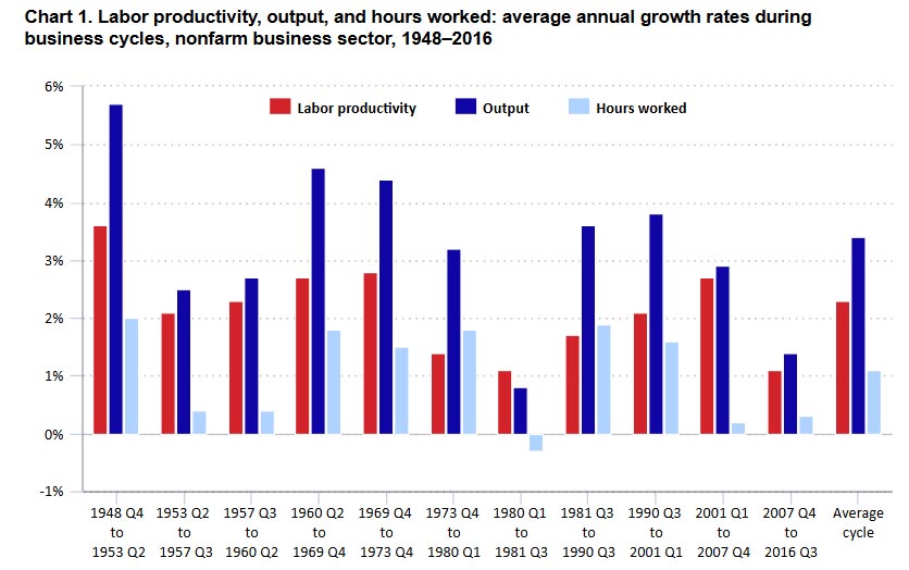
While hours growth during the current business cycle was 0.8 percentage point below its business cycle average of 1.1 percent, output growth was 2.0 percentage points below its business cycle average of 3.4 percent. So, although both hours and output grew at below-average rates during this cycle, the fact that output grew notably slower than its historical average is what yields the historically low labor productivity growth rate of 1.1 percent.

Now let us look more deeply into the output and hours data and see how each has been moving during the current business cycle relative to its historical trend and how each of these series is reflected in the low labor productivity growth of this cycle.

Output growth in the current business cycle

The below-average rate of output growth in the current business cycle had contributions from both phases of the cycle: the Great Recession and the subsequent recovery. The Great Recession had the largest total decline in output of any recession in the post–WWII era (a 6.7-percent overall decline). Following that historic decline, the recovery has had the lowest output growth rate (2.6 percent per year) of any recovery since 1947. These two factors have combined to yield an output growth rate for this cycle (1.4 percent per year) that is very low by historical standards. Only the brief 1980 cycle had a lower rate, and all nine other cycles had growth rates of at least 2.5 percent, well above the output growth rate of the current cycle. (Compare the dark blue bars in chart 1.)

A key aspect of the recovery thus far is that, not only has output growth been well below historical trends, but it is even further behind the growth rates necessary to overcome the effect of the massive decline in output during the Great Recession. To counteract such a large decline and lift the current cycle’s growth rate back up to historical averages, output would have had to grow much faster than average during the recovery. But output has done the opposite thus far, growing more slowly than average during the recovery.

You may be wondering how large of an output growth rate during the recovery would have been required to lift this business cycle’s output growth back up to the long-term trend. The answer is that it would have taken a 5.5-percent growth rate up to this point in the current recovery to lift this cycle’s output growth rate up to the 3.7-percent long-term rate registered from 1947 to 2007. That 5.5-percent rate is 2.9 percentage points higher than the actual 2.6-percent growth rate of the recovery. We can also calculate the rate necessary to lift this cycle’s growth rate to that of the more recent trends. For example, to attain the 2.9-percent growth rate of the last business cycle—from the first quarter of 2001 to the fourth quarter of 2007—the current recovery would have needed a 4.5-percent output growth rate—1.9 percentage points higher than the growth rate posted thus far in this business cycle.

The gap between the current output series and historical trend rates can be seen in chart 2. The output series of the current business cycle is shown by the solid dark-blue line, and the dashed and dotted dark-blue lines show the trends in output for the entire historical period and the last business cycle. Comparing the current output series with the long-term output growth trend from 1947 to 2007 (the dashed dark-blue line), we can see that the current series lies well below this trend line and that the gap between the series has widened since the end of the recession. Put in dollar terms, the gap between the actual output and this hypothetical output if it had continued to follow the 1947-to-2007 output trend during this cycle is now more than $2.7 trillion, or over $22,900 in lost annual output per job in the nonfarm business sector. Comparing the current series with the trend rate from the previous business cycle (the dotted dark-blue line) also reveals that the output gap has widened since the end of the recession, although by less than the full historical trend indicates.

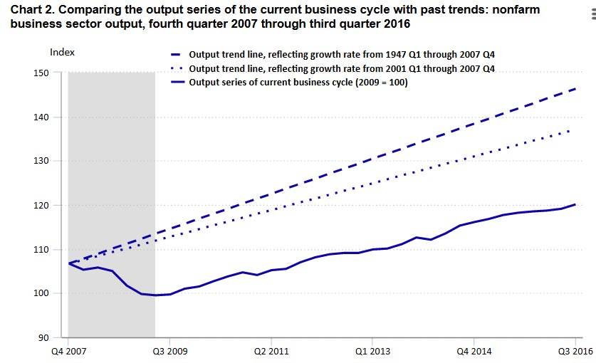
These historical comparisons make it clear that the shock to output growth which took place during the Great Recession has not been resolved. The fact that output growth has not risen above 3.2 percent in any single year since the recession underlines the fact that the higher-than-average growth rates which would be necessary for the U.S. economy to climb back to pre-recessionary trends have not been present during this recovery. At this point in the recovery, it would require a dramatic increase in output growth rates to resolve this situation.

Hours growth in the current business cycle

Just as with output growth, we can perform a long-term comparative analysis on the hours growth in the current business cycle. During the Great Recession, hours sustained an overall decline of 9.9 percent (or 19.4 billion labor hours) from the business cycle peak in the fourth quarter of 2007 until its subsequent low point in the third quarter of 2009. Following that decline, hours have grown during this recovery at an average annual rate of 1.9 percent. Chart 3 shows how hours have fared throughout this business cycle relative to historical trends. The first thing you might notice is that there is no gap in hours growth between this business cycle and the cycle that ran from the first quarter of 2001 to the fourth quarter of 2007. In fact—as can be seen by looking at the right side of the chart—hours growth in the current cycle (the solid light-blue line) has already surpassed that of the 2001–07 period (the dotted light-blue line). As of the third quarter of 2016, hours have grown during this business cycle at an annual rate of 0.3 percent, compared with 0.2-percent growth over the last cycle. The 1.9-percent hours growth rate during the current recovery was key to closing the gap in growth between this cycle and the last one.

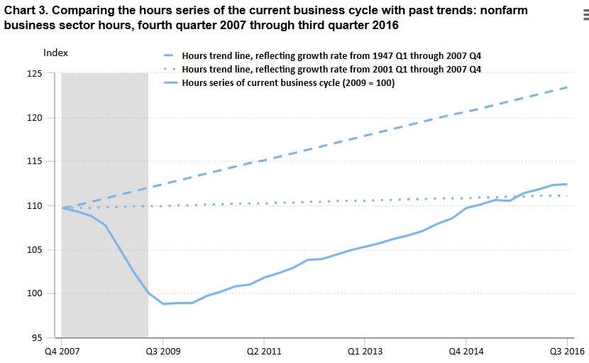
You might also notice that the slope of the hours line of the current recovery is slightly steeper than the slope of the line representing the 1947-to-2007 trend (the dashed light-blue line). This relationship indicates that the current recovery’s hours growth has outpaced its long-term historical trend and has thus helped this business cycle’s growth rate begin to catch up to that long-term trend. However, a gap remains between the overall growth of the current cycle and hours growth over the long-term historical period. In order for the current-cycle hours growth to match the trend from 1947 to 2007, hours would have needed to grow 3.2 percent during the recovery thus far; this rate is 1.3 percentage points above the current-recovery rate of 1.9 percent. So, we can say that, although the hours growth rate up to this point in this business cycle is similar to the rate from the last cycle, hours have still grown at rates below the long-term historical trend.

Overall, hours have recovered much better than output, having fully caught up to the growth rate of the last business cycle and even having made some progress toward catching up to the long-term trend. Output, in contrast, is still far behind both its recent and its long-term trend, and has made no progress in catching up to those trends during its recovery, as is shown by the substantial gap in growth remaining as of the third quarter of 2016—a gap that is even larger than that existing at the end of the Great Recession. (See chart 2.)

Labor productivity growth in the current business cycle

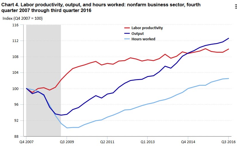
Now let us look at how the growth in output and the growth in hours combine to yield the historically low labor productivity growth of the current business cycle. Chart 4 reveals that, through most of the Great Recession, labor productivity was relatively flat, as output and hours were declining simultaneously. However, as the recession was ending, productivity shot up when output stabilized while hours continued to fall. In fact, nearly half of the overall productivity growth during the current business cycle occurred in just the period from the fourth quarter of 2008 to the fourth quarter of 2009. The high productivity growth of that yearlong period comes from the fact that the largest overall output decline (–6.7 percent) since the Great Depression was surpassed by an even larger decline in hours worked (–9.9 percent). This example shows that, although productivity grows when output rises by a larger amount than hours, productivity also grows when output declines by a smaller amount than hours.

Following the spike in productivity which occurred in 2009, both output and hours grew at rates that were relatively similar to one another during the remainder of the recovery, resulting in the very low productivity growth seen during this period. Over the last 5 years shown in chart 4, labor productivity grew at an average rate of just 0.7 percent, with output growing 2.6 percent and hours growing 1.9 percent. The 0.7-percent labor productivity growth rate during these years is less than one-third the long-term rate of productivity growth of 2.3 percent posted from 1947 to 2007.

Just as we saw with output and hours, we can see how labor productivity has performed in the current business cycle relative to historical trends. Chart 5 shows labor productivity during this business cycle (the solid red line) compared with trends for the same historical periods that we used to analyze output and hours. Through most of the Great Recession, labor productivity lagged behind historical growth rates, but then it achieved above-average gains coming out of the recession and into the early quarters of the recovery. The U.S. economy actually caught up to the long-term historical trend (the dashed red line) in the fourth quarter of 2009, although it was still slightly behind the trend from the last cycle (the dotted red line) at that point. However, after 2010, productivity growth stagnated and a substantial deficit relative to historical trends developed over the next 5 years. By the third quarter of 2016, labor productivity in the current business cycle had grown at an average rate of just 1.1 percent, well below the long-term average rate of 2.3 percent from 1947 to 2007 and even further behind the 2.7-percent average rate over the cycle from 2001 to 2007.

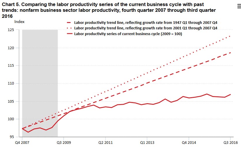
Ultimately, the fact that labor hours have outpaced their historical trend during this recovery while output has fallen further behind its historical trend is what yields the low productivity of the current cycle. This combination is illustrated on the right side of chart 5, where the stagnation of labor productivity growth is plainly visible.

Dramatic gains in labor productivity growth would be required in coming years to counteract the stagnation of recent years and lift the series back up to the long-term historical trend. For example, it would require a constant productivity growth rate of 7.7 percent during each of the next 2 years in order to lift the labor productivity growth of the current cycle back up to the historical trend rate seen from 1947 to 2007. This rate of growth would be 7 times that of this business cycle thus far, and 11 times the rate experienced during the last 5 years.

Wage gap growth in the current business cycle

Sluggish productivity growth has implications for worker compensation. As stated earlier, real hourly compensation growth depends upon gains in labor productivity; thus, low labor productivity growth can limit potential gains for workers. During the current business cycle, real hourly compensation (the gold bars in chart 6) has increased 0.7 percent, which is low by historical standards. The rate is lower than the average real hourly compensation growth rate of 1.7 percent observed during other business cycles. The rate is also below the rates of all other cycles, except for a brief six-quarter cycle in the early 1980s. Note also that the low growth rate of the current business cycle is a near-continuation of the similarly low growth rate of the early-2000s cycle (0.8 percent).

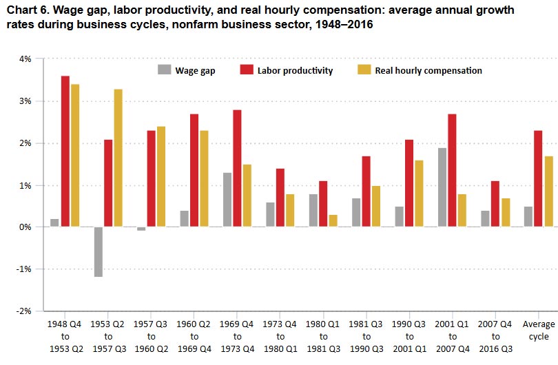
There is, however, one interesting difference between the low real hourly compensation growth in the current business cycle and the low real hourly compensation growth in the last cycle. The “wage gap”—defined as the difference in the growth rates of labor productivity and real hourly compensation —for the current cycle is much smaller, at just 0.4 percent. (Compare the gray bars in chart 6.) In fact, the current U.S. business cycle is exhibiting the smallest wage gap since the 1960s. Note, however, that it has been the historically low productivity growth alone that has shrunk the wage gap in the current business cycle, as there were no improvements in real hourly compensation growth relative to the rates from recent cycles.

Looking forward

The historically low rate of labor productivity growth during the current business cycle has limited gains in living standards for Americans during this period. U.S. workers have had to work more hours in order to produce the current supply of goods and services than would have been the case with higher productivity growth. In addition, low productivity growth has limited potential gains in worker compensation and in shareholder profits; these income gains are ultimately dependent upon gains in goods and services produced per hour of work. Americans would be wise to pay attention to productivity trends in coming years, as these trends will figure prominently in our lives and in the lives of future generations.

The Trump effect on bond markets and trade

From Investor Daily.

The Australian bond market is likely to feel the effects of US President Donald Trump’s protectionist trade stance both directly and indirectly, writes Nikko Asset Management’s James Alexander.

The emergence of China is clearly of great importance to the economic fortunes of Australia, and as a result it may be tempting to downplay, or even overlook, President Trump’s agenda and its impact on Australia.

While our largest import and export partner is now China, Australia will still be impacted by US trade policy both directly and, perhaps more importantly, indirectly.

The difficulty for investors, however, is the general uncertainty around future US trade policy, and the impact the Trump administration will have on financial markets.

Uncertainty around trade

While most of President Trump’s comments so far have been directed at China and Mexico, we do know that he is not a fan of trade deals negotiated by others.

Trade deals he has criticised in which Australia has been involved include the Trans-Pacific Partnership (TPP), from which the US has just withdrawn, and the North American Free Trade Agreement (NAFTA).

The essential message here is that these are bad deals for the US, as opposed to future Trump-negotiated deals, which will of course be good for the US.

It is likely to be some time before we can reasonably assess the impact of changes to US trade policy with Australia directly, given their larger trade relationships are most certainly ahead of us in the queue.

This brings us to the indirect but significant impact of the US’ future trade relations with our biggest trading partner, China.

A tit-for-tat trade war is likely to be harmful to both the US and China, with Australia most certainly suffering some collateral damage.

It is too early to tell how this relationship will unfold but the early signs are not great, with President Trump taking every opportunity to criticise China.

These two economic heavyweights have plenty of tools to ‘penalise’ each other on trade, which could potentially hurt Australian trade in the process.

Rising bond yields

The other broad area where the impact of a Trump presidency is likely to be felt is in financial markets – more specifically, bond yields and foreign exchange rates.

Australia’s bond yields have historically been strongly correlated with US Treasury yields and this is likely to continue.

If the Trump agenda of lower taxes, increased infrastructure spending and more protectionist trade policy prove to be inflationary as we expect, US interest rates and bond yields are likely to be headed higher.

Australian bond yields will surely follow, as Commonwealth bond yields must remain globally competitive to ensure international investors continue to support our borrowing needs.

Another widely discussed by-product of Trump’s agenda is a stronger US dollar.

While the Australian dollar has fallen by around 2.5 per cent against the American currency, it has actually risen slightly on a trade-weighted basis since the presidential election in November.

This divergence, should it continue, will be one to watch carefully.

While a weaker Australian dollar would indeed help to counter any negative impact from higher bond yields, weakness that is mainly isolated to the US dollar is not nearly as helpful as weakness on a trade-weighted basis.

James Alexander is the co-head of global fixed income and head of Australian fixed income at Nikko Asset Management.

The Financing of Nonemployer Firms

From The St. Louis Fed Blog.

Nonemployer firms that applied for financing were more likely to operate at a loss, according to the recently released 2015 Small Business Credit Survey: Report on Nonemployer Firms.

This report, produced jointly by the Federal Reserve banks of St. Louis, Atlanta, Boston, Cleveland, New York, Philadelphia and Richmond, examined trends in businesses with no employees other than the owners. As the report noted, these businesses make up nearly 80 percent of all U.S. firms.

Applying for Financing

The report noted that 32 percent of survey respondents said they applied for financing in the previous 12 months. Among those who applied, the most common reason (66 percent) was to expand the business or to take advantage of a new opportunity. The next most common reason (38 percent) was to cover operating expenses. (Respondents could select multiple answers.)

Among those businesses that did not apply for financing, the top three reasons were:

  • Debt aversion (33 percent)
  • Already had sufficient financing (30 percent)
  • Believed they would be turned down (25 percent)

Profitability: Applicants vs. Nonapplicants

As the report noted: “Collectively, applicants were less profitable than the nonapplicants.” The figure below shows the difference.

profitability of small businesses that applied for financing

Financing Approval

Among firms that applied for financing, 41 percent were not approved for any of the funding they sought. The percentages of firms not receiving any funding grew smaller as firms grew larger: 48 percent of firms with less than $25,000 in revenue did not receive any funding, while only 28 percent of firms with revenues greater than $100,000 did not receive funding.

About 71 percent of firms received less financing than the amount sought. When asked about the primary impact of this financing shortfall, the top response (33 percent) said the firm had to delay expansion. Other top answers were that they used personal funds (22 percent), were unable to meet expenses (18 percent) and passed on business opportunities (13 percent).

Additional Resources