Aligning Growth Policy Levers

Glenn Stevens gave an address to the Economic Society of Australia in Brisbane where he discussed the need to align policy levers to drive growth and the limits of monetary policy.

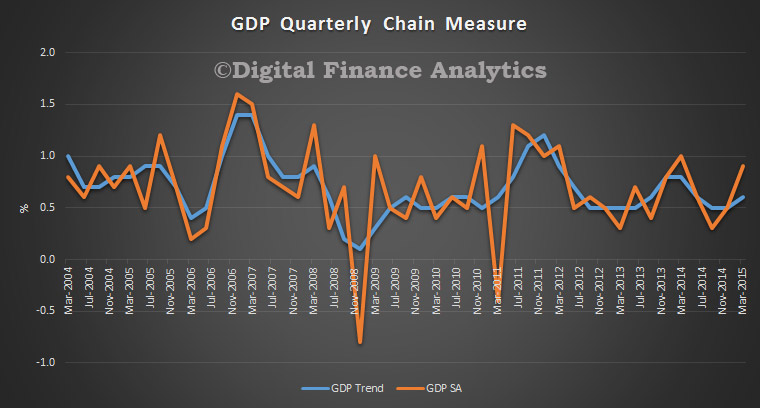
The latest edition of the Australian National Accounts, released last week, shows the picture. The quarterly growth figure was stronger than what had been embodied in our forecasts in the May Statement on Monetary Policy, though that comes after a weaker-than-expected outcome in the previous quarter. Some of the strength resulted from unusually high export shipments of resources, which were less disrupted by weather conditions in the ‘cyclone season’ than has often been the case in the past. Indications are that this pace of growth wasn’t repeated in the June quarter, when shipments of coal in particular were affected by weather disruptions on the east coast.

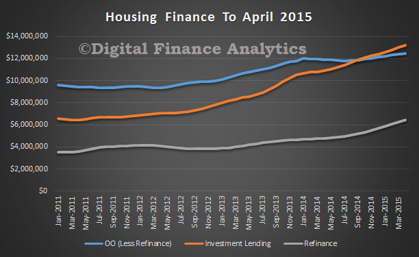
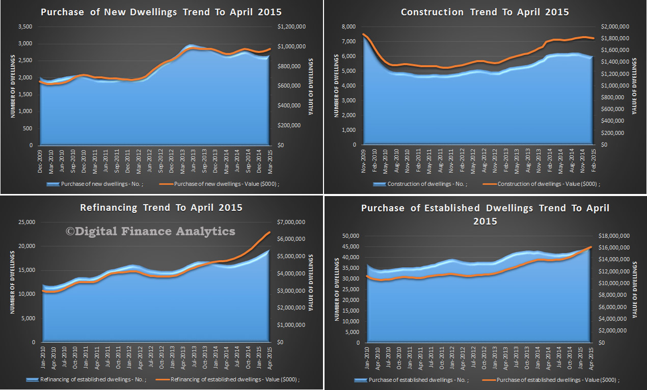
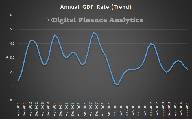
Taking the results over the past four quarters, growth was ‘below trend’. Export volume growth contributed strongly, while domestic final demand increased by a bit under 1 per cent, which is quite a weak result. Housing construction rose strongly, and consumer spending over the year rose by more than real household income (that is, the saving rate fell). Both these results owe a good deal to low interest rates and rising asset values.

But other components of demand were weak. Business investment fell substantially, with mining investment falling quickly and, as best we can tell, non-mining capital spending also weak. Public final spending didn’t grow at all. Public investment spending fell by 8 per cent over the past year.

Overall, these outcomes are weaker that what, two years ago, we expected would be happening by now. Back then, the two-year-ahead forecast was for annual GDP growth to be in a range of 2½ to 4 per cent by mid 2015. The width of that range reflected the normal size of error margins, coupled with the inevitable uncertainty about the timing of when some components of demand outside of mining might strengthen, and the judgement that if accommodative monetary policy really was held in place for several years (which was a key assumption behind those forecasts), activity could at some point start to pick up quite quickly. It will be three months before we get the national accounts data for the June quarter, but at this point, with three of the four quarters available for the year to June 2015, it would appear that the outcome will be either right at the bottom of the range predicted two years ago or, more likely, a bit below it.

Of course, forecasts are hardly more than educated guesswork and two-year-ahead forecasts are even less reliable. That there are inevitably forecast errors is neither surprising nor new, and it is not any more concerning per se now than it always has been. This is far from the biggest forecast error I’ve seen over my three decades in this game.

But it is nonetheless useful to see what we can learn from those errors.

The following points are prominent:

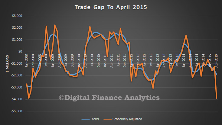
  • The terms of trade, which two years ago were assumed to fall, have in fact fallen further – they are about 12 per cent lower than the assumed path. That means national income is lower, which means spending power is lower.
  • The exchange rate, which at that time was above parity against the US dollar, and was assumed to stay there, is now about 25 per cent lower. It has moved in the same direction as the terms of trade, which is normal.
  • The lower exchange rate has helped to produce a contribution to growth from ‘net exports’ much greater than earlier forecast, while that from domestic demand has been much weaker. The latter is mainly spread across non-mining business investment and weaker government spending, together with softer consumption on account of lower incomes. One thing which is not very different from the forecast from two years ago is that mining sector capital spending is falling sharply.
  • Because the net effect of the above factors is that GDP growth has been on the weaker side of expectations, the unemployment rate is about half a percentage point higher than forecast two years ago. Consistent with that, growth in wages is, as you would expect, lower than forecast.
  • Headline inflation is lower than forecast, largely because of the recent fall in oil prices. Underlying inflation is within the 2–3 per cent range that had been forecast. Again, the depreciation of the exchange rate has been a factor here.
  • The cash rate is 75 basis points lower than assumed two years ago, as monetary policy has used the room provided by contained inflation to try to do more to help growth. Lending rates have fallen on average by about 100 basis points over that period. This has produced a stronger result for housing construction than forecast and will also have contributed to the rise in dwelling prices.

In summary, the economy has in several important respects followed a different track from the one expected a couple of years ago. That is partly because conditions in the world economy were different from what had been expected and partly because several domestic factors were different.

Some in-built responses have been in evidence. For example the decline in the exchange rate, even if not by as much as we might have expected, has had the effect of supporting growth and keeping inflation from falling as much as it might have done. And, of course, monetary policy has also responded to the evolving situation, consistent with the Reserve Bank’s mandate. These responses have had the effect of lessening the extent to which growth and inflation have differed from the outcomes expected two years ago, but haven’t managed to eliminate those differences entirely, at least in the case of output growth.

The slowing in wage growth in response to soft labour market conditions has also undoubtedly helped to hold employment up. In fact wage growth appears to be somewhat lower than previous relationships between wages and unemployment would suggest. This may be a sign of increased price flexibility in the labour market and could help to explain why employment recently has looked a little higher relative to estimated GDP than might have been expected. These hypotheses can be advanced only tentatively, though, until we have more data.

Looking ahead, the most recent forecasts suggest that growth rates will be similar to those we have observed recently for a while yet. Residential investment will reach new highs over the period ahead. Household consumption is expected to record moderate growth. With national income growth reduced by a falling terms of trade, this requires a modest decline in the saving rate. It doesn’t seem reasonable to expect much more from consumption growth than that.

Resources sector investment has a good deal further to fall yet over the next two years. Other areas of investment seem very low and while I would have expected that by now these would have been showing signs of strengthening, the most recent indications are for, if anything, a weakening over the year ahead. Public final spending has not been growing and fiscal consolidation still has some way to run. Under the current macroeconomic conditions, it would seem inappropriate for governments to seek additional restraint here in the near term.

Inflation is likely to remain low. Growth in labour costs is very low and some of the forces that were pushing up certain administered prices have started to reverse. So even if the exchange rate were to fall further, which in my view it needs to, we seem unlikely to have a problem with excessive inflation.

Putting all that together, as things stand, the economy could do with some more demand growth over the next couple of years.

Of course, these are forecasts. They might be wrong. In fact, they will be wrong, in some dimension or other. Our published material goes to some lengths to articulate a range of ‘risks’. It is easy to think of ‘downside’ ones in the current mood of determined pessimism.

But it is not entirely impossible to think of upside ones as well. A further fall in the exchange rate, which is not assumed in the forecasts, would add both to growth and prices. If one thinks that such a decline at some point is likely, that constitutes an ‘upside’ risk. Of course, the list of countries that would prefer a lower exchange rate is a long one and we can’t all have it.

That being so, we might give some thought to trying to create some upside risks to the growth outlook through policy initiatives. The Reserve Bank will remain attuned to what it can do, consistent with the various elements of its mandate – including price stability, full employment and financial stability. We remain open to the possibility of further policy easing, if that is, on balance, beneficial for sustainable growth.

The temptation, of course, is to presume outcomes can be fine-tuned by policy settings and that we can simply dial up more or less demand in short order to avoid deviations from some ideal path. Reality is inevitably more messy than that and has not always been kind to such fine-tuning notions. As it is, some observers think monetary policy has done too little, while others think it already has done way too much. I think it has been about right for the circumstances.

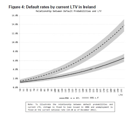
But the bigger point is that monetary policy alone can’t deliver everything we need and expecting too much from it can lead, in time, to much bigger problems. Much of the effect of monetary policy comes through the spending, borrowing and saving decisions of households. There isn’t much cause from research, or from current data, to expect a direct impact on business investment. But of all the three broad sectors – households, government and corporations – it is households that probably have the least scope to expand their balance sheets to drive spending. That’s because they already did that a decade or more ago. Their debt burden, while being well serviced and with low arrears rates, is already high. It is for this reason that I have previously noted some reservations about how much monetary policy can be expected to do to boost growth with lower and lower interest rates. It is not that monetary policy is entirely powerless, but its marginal effect may be smaller, and the associated risks greater, the lower interest rates go from already very low levels. I think everyone can see that.

If I am correct about this, it really is very important that other policies coalesce around a narrative for growth. In this regard, I think the Government is on the right track in not seeking to compensate for lower revenue growth by cutting spending further in the short run. Of course, some resolution of long-run budget trends is still going to be needed to sustain confidence and that will not be an easy conversation.

Meanwhile, as often remarked, infrastructure spending has a role to play in sustaining growth and also in generating confidence. I am doubtful of our capacity to deploy this sort of spending as a short-term countercyclical device. The evidence of history is that it takes too long to start and then too long to stop. But it would be confidence-enhancing if there was an agreed story about a long-term pipeline of infrastructure projects, surrounded by appropriate governance on project selection, risk-sharing between public and private sectors at varying stages of production and ownership, and appropriate pricing for use of the finished product. The suppliers would feel it was worth their while to improve their offering if projects were not just one-offs. The financial sector would be attracted to the opportunities for financing and asset ownership. The real economy would benefit from the steady pipeline of construction work – as opposed to a boom and bust. It would also benefit from confidence about improved efficiency of logistics over time resulting from the better infrastructure. Amenity would be improved for millions of ordinary citizens in their daily lives. We could unleash large potential benefits that at present are not available because of congestion in our transportation networks.

The impediments to this outcome are not financial. The funding would be available, with long term interest rates the lowest we have ever seen or are likely to. (And it is perfectly sensible for some public debt to be used to fund infrastructure that will earn a return. That is not the same as borrowing to pay pensions or public servants.) The impediments are in our decision-making processes and, it seems, in our inability to find political agreement on how to proceed.

Physical infrastructure is, of course, only part of what we need. The confidence-enhancing narrative needs to extend to skills, education, technology, the ability and freedom to respond to incentives, the ability to adapt and the willingness to take on risk. It is in these areas too, where there are various initiatives in place or planned, but which often do not get enough attention, that we need to create a positive dynamic of confidence, innovation and investment.

That is the upside we need to create.

Housing Finance Up In April Is Investment Driven

The ABS released their Housing Finance Statistics to April 2015 today. The trend estimate for the total value of dwelling finance commitments excluding alterations and additions rose 1.4% to $32,109 m.

Investment housing commitments rose 1.4% and owner occupied housing commitments rose 1.3%. This is a strong result, and ahead of expectations. We suspect investors are bringing purchase decisions forwards ahead of possible anticipated lending tightening later. Further evidence that the dial needs to be turned back.

Looking at the trends, more than half of new loans (excluding refinance were for investment purposes, and the value of refinancing continued to track higher as borrowers move on to the new lower rate offers.

HousingFinanceTrendsApril2015In trend terms, the number of commitments for owner occupied housing finance rose 0.7% in April 2015. In trend terms, the number of commitments for the purchase of new dwellings rose 1.1% and the number of commitments for the purchase of established dwellings rose 0.8%, while the number of commitments for the construction of dwellings fell 0.2%

HousingFinanceApril2015In original terms, the number of first home buyer commitments as a percentage of total owner occupied housing finance commitments rose to 15.2% in April 2015 from 15.1% in March 2015. However, in NSW it was lower, at 11%, in an environment where investment lending is hot.

FTBApril2015However, the true first time buyer picture is more complex with a continued lift in FTB investors, as shown in the DFA adjusted picture. More than 4,000 FTB investors joined the ranks this month, a record, compared with about 7,000 OO FTB. If this continues, we expect investors to overtake OO FTB by the end of the year.

FTBAdjustedApril2015

Solvency Or Bust?

Public debt is a normal part of a government’s finances, but too much debt can have serious consequences for a country. During a seminar at the IMF-World Bank Meetings, Helen Clark, one former head of state, who left office with public finances in good standing, explains how her administration in New Zealand succeeded where others have so often failed.

Link to Podcast

Trade Gap Surprise – Deficit of $3.8 billion

The ABS published the April International Trade in Goods and Services to April 2015. In trend terms, the balance on goods and services was a deficit of $1,883m in April 2015, an increase of $292m (18%) on the deficit in March 2015. However,  in seasonally adjusted terms, the balance on goods and services was a deficit of $3,888m in April 2015, an increase of $2,657m (216%) on the deficit in March 2015. This is a significant “blip” and seems to be caused by a couple of specific one-off items, including loss of exports caused by bad weather, and the purchase of a large piece of machinery.

TradeGapApril2015In seasonally adjusted terms, goods and services credits fell $1,561m (6%) to $25,659m. Non-rural goods fell $1,271m (8%) partly driven by coal, coke and briquettes, down $859m (22%) as a result of the temporary closure of ports due to severe weather conditions. Non-monetary gold fell $306m (22%), rural goods fell $31m (1%) and net exports of goods under merchanting fell $5m (15%). Services credits rose $52m (1%).

In seasonally adjusted terms, goods and services debits rose $1,096m (4%) to $29,547m. Capital goods rose $546m (10%) driven by imports of machinery and industrial equipment, up $1,232m (69%). Intermediate and other merchandise goods rose $371m (4%) and consumption goods rose $314m (4%). Non-monetary gold fell $91m (24%). Services debits fell $43m (1%).

Retail Trade Trend Up 0.3% In April

The latest Australian Bureau of Statistics (ABS) Retail Trade figures show that Australian retail turnover was relatively unchanged in April (0.0 per cent) following a rise of 0.2 per cent in March 2015, seasonally adjusted. In monthly terms the trend estimate for Australian retail turnover rose 0.3 per cent in April 2015 following a 0.3 per cent rise in March 2015. Though the seasonally adjusted result was relatively unchanged this month, the trend result for April 2015 is up 4.4 per cent compared to April 2014.

In seasonally adjusted terms there were rises in cafes, restaurants and takeaway food services (0.8 per cent) and clothing, footwear and personal accessory retailing (1.3 per cent). Household goods retailing was relatively unchanged (0.0 per cent). There were falls in other retailing (-1.0 per cent), food retailing (-0.1 per cent) and department stores (-0.7 per cent).

In seasonally adjusted terms there were rises in Victoria (0.5 per cent), the Australian Capital Territory (0.6 per cent), South Australia (0.1 per cent) and the Northern Territory (0.1 per cent). New South Wales was relatively unchanged (0.0 per cent). There were falls in Queensland (-0.6 per cent), Tasmania (-0.9 per cent) and Western Australia (-0.1 per cent).

Online retail turnover contributed 3.0 per cent to total retail turnover in original terms.

GDP Beats Expectations In March Quarter

Latest Australian Bureau of Statistics (ABS) figures show that GDP, in seasonally adjusted chain volume terms, grew 0.9 per cent in the March quarter 2015. The consensus expectation was 0.7%.

GDPMar2015Chain

Trend GDP growth was 0.6% in the last quarter, making an annual 2.2%.

GDPMarch2015Annual Net exports contributed 0.5 percentage points to GDP growth. Household final consumption expenditure and Changes in inventories each contributed 0.3 percentage points to GDP growth. This was offset by a -0.3 percentage point contribution from Gross fixed capital formation.

The industries which drove GDP growth in the March quarter were Mining and Financial and insurance services. Mining contributed 0.3 percentage points and Financial and insurance services contributed 0.2 percentage points.

The March quarter saw the Terms of trade decrease 2.9 per cent in seasonally adjusted terms.


RBNZ Issues Consultation On LVR Rules For Auckland Residential Property Investors

The NZ Reserve Bank has published a consultation paper about proposed changes to the rules that banks must follow for high-LVR mortgage loans.

The proposals were announced in the Reserve Bank’s Financial Stability Report released on 13 May 2015. They would mean investors in Auckland property would generally need a 30 percent deposit if they’re borrowing for a property, while home buyers outside Auckland would see increased availability of high-LVR mortgages.

The specific proposals are to:

  • Restrict property investment residential mortgage loans in the Auckland region at LVRs of greater than 70 percent to 2 percent of total property investment residential mortgage commitments in Auckland.
  • Retain the existing speed limit of 10 percent for other residential mortgage lending, as a proportion of total non-property investment residential mortgage commitments, in the Auckland region at LVRs above 80 percent.
  • Increase the speed limit on residential mortgage lending at LVRs above 80 percent outside of Auckland to 15 percent of residential mortgage commitments outside Auckland.

A number of loan categories are exempted from LVR speed limits, and these exemptions will be retained under the proposed policy changes. Specifically, loans that are made as part of Housing New Zealand’s Welcome Home Loan scheme, and loans that are made for the purpose of refinancing an existing mortgage loan, moving house (without increasing borrowing amount), bridging finance or constructing a new dwelling will continue to be exempt from the policy.

The paper also offers further evidence on the different risk profiles of investment versus owner occupied loans in a down turn, including data from experiences in Ireland.

“Residential property investment loans appear to have relatively low default rates during normal economic circumstances. However, the Reserve Bank has looked at evidence from extreme housing downturns during the GFC, and this clearly indicates that default rates can be higher for investor loans than for owner occupiers in severe downturns. For example, as shown in table 1, forecast loss rates on Irish mortgages were nearly twice as high for investors as for owner-occupiers. Similarly, actual arrears rates were about twice as high for investor loans (29.4 percent) than for owner occupied loans (14.8 percent) as at December 2014. Furthermore, studies which have separately estimated default rates by LVR for investor loans and owner occupier loans suggest that investor loans are substantially riskier at any given LVR. The data  shows an estimate of default rate based on current LVR. For example, if a loan was initially written at a 70 percent LVR and then prices fell 30 percent, the loan would appear in the chart below as LTV=100. This would have a mildly increased rate of default compared to a low-LVR loan for an owner occupier. But for an investor, the rate of default would be higher, and would have increased more sharply as a result of a given decline in house prices.”

RBNZ-Ireland-DefaultsNote: PDH is principal dwelling house, BTL is buy to let. LTV (loan to value ratio) is conceptually the same as LVR, but this dataset uses the current LTV (after the sharp falls in house prices) rather than origination LTV.

The consultation will run until 13 July. The Reserve Bank expects to publish a summary of submissions and final policy position in August, with revised rules taking effect from 1 October.

The Reserve Bank proposes that the policy changes take effect from 1 October 2015. This relatively long notice period is to allow banks to make the necessary systems changes in order to properly classify new lending. There is a risk that a notice period of this length could lead to some Auckland property investors rushing in to beat the policy changes. However, our expectation is that banks will observe the spirit of the proposed restrictions, and will act to curtail lending at LVRs of above 70 percent to Auckland property investors well in advance of 1 October.

Currently, compliance with the LVR policy is measured over a three-month rolling window for banks with monthly lending of over $100m, and over a six-month rolling window for banks with monthly lending of less than $100m. At the time that LVR restrictions were first introduced, all banks were provided with an initial six-month measurement period. This was done to accommodate outstanding pre-approved loans, and recognised the relatively short notice period provided. A longer first measurement period does not appear to be warranted for this change to the restriction, given more than four months’ notice of an intention to change the restriction. Further, the low speed limit for Auckland property investment mortgage lending does not provide much scope to smooth lending over a longer measurement period.

US Economic Outlook and Monetary Policy

A speech by Governor Lael Brainard at the Center for Strategic and International Studies, Washington, D.C. on “The U.S. Economic Outlook and Implications for Monetary Policy” suggests that whilst the US economic outlook is patchy, interest rates will rise.

This spring marks the end of the Federal Reserve’s calendar-based forward guidance and the return to full data dependency in the setting of the federal funds rate. So it is notable that just as policymaking is becoming more anchored in meeting-by-meeting assessments of the data, the data are presenting a mixed picture that lends itself to materially different readings.

No doubt, bad weather, port disruptions, and statistical issues are responsible for some of the softness in first-quarter indicators of aggregate spending. Indeed, it may be that the dismal estimate by the Bureau of Economic Analysis of the annualized change in first-quarter gross domestic product (GDP), negative 0.7 percent, is principally an extension of the pattern, seen for several years, of significantly slower measured GDP growth in the first quarter followed by considerably stronger readings during the remainder of the year. In that case, it would be appropriate to minimize the importance of the first-quarter estimate in judging the likely path of the economy over the remainder of the year.

But there may be reasons not to ignore the recent readings entirely. First, the limited data in hand pertaining to the second quarter do not suggest a significant bounceback in aggregate spending, which we would expect if all of the weakness in the first quarter were due to transitory factors. Private-sector forecasts of second-quarter growth are centered around 2-1/2 percent, while the Federal Reserve Bank of Atlanta’s GDPNow forecast, which was quite accurate in its prediction of the first estimate of first-quarter GDP growth, is projecting second-quarter GDP growth of only 0.8 percent.

Second, it would not be the first time this recovery has proceeded in fits and starts. The underlying momentum of the recovery has proven relatively susceptible to successive headwinds, which have kept overall economic growth well below the average pace of previous upturns.

My own reading is that earlier, more optimistic growth projections may have placed too much weight on the boost to spending from lower energy prices and too little weight on the negative implications for aggregate demand of the significant increase in the foreign exchange value of the dollar and large decline in the price of crude oil.

Based on today’s picture of moderate underlying momentum in the domestic economy and the likelihood of continued crosscurrents from abroad, the process of normalizing monetary policy is likely to be gradual. It is also important to remember that the stance of monetary policy will remain highly accommodative even after the federal funds rate moves off the effective lower bound, because the real federal funds rate will initially still be low and because of the elevated size of the Federal Reserve’s balance sheet and the associated downward pressure on long-term rates. Moreover, the FOMC has stated clearly that it will reduce the size of the balance sheet in a gradual and predictable manner starting at an appropriate time after liftoff, which will depend on how economic and financial conditions evolve.

In summary, the string of soft data in the first quarter raises some questions about the contours of the outlook. While it is possible that residual seasonality and temporary factors were responsible, it would be difficult, based on the data available today, to dismiss the possibility of a more significant drag on the economy than anticipated from foreign crosscurrents and the negative effects of the oil price decline, along with a more cautious U.S. consumer. This possibility argues for giving the data some more time to confirm further improvement in the labor market and firming of inflation toward our 2 percent target. But while the case for liftoff may not be immediate, it is coming into clearer view. When that time comes, the policy path will be highly attuned to incoming data and not on a preset course, and it is important to be mindful of the possibility of volatility as markets adjust to a change in the stance of policy. Thus, the FOMC will continue communicating as clearly as possible regarding the outlook and the factors underlying its policy determinations.

The Budget is Still Unfair – The Conversation

From The Conversation’s “Looking inside the sausage machine.” NATSEM’s analysis of the 2015-16 federal budget, the same as used by the Howard and Rudd–Gillard governments as a policy tool, has been likened by Treasurer Joe Hockey to a sausage machine.

What makes Hockey’s analogy particularly striking is its applicability to this year’s budget process. While the government threw away the very toughest bits of gristle from last year, a number of the most unpalatable cuts are still in the mince, plus some added sweeteners.

Like last year, we have made some calculations showing the impact of the budget measures on disposable income in July 2017, once most of the proposed indexation pauses have taken effect.

Our assumptions are conservative. We consider as status quo the repeal of changes to income tax rates and the low-income tax offset. Like last year, we do not factor in the abolition of the Schoolkids Bonus, or the Income Support Bonus, because this was not strictly speaking a budget measure.

Restricting eligibility for Family Tax Benefit Part B, or FTB-B, may lead to substantial losses of disposable income for families with school-aged children – even before the Schoolkids Bonus is taken away. Our figures show that a couple with two children aged 11 and 8, where one parent earns A$60,000 per year, would lose A$84.43 per week, or 7.4% of disposable income. A single parent with one child aged 8 and no private income stands to lose A$49.93 per week, or 10.9% of disposable income.

Pausing indexation of all FTB payment rates affects the most vulnerable families. A couple with no private income and one 3-year-old child would lose A$11.24 per week, or 1.8% of disposable income, while a single parent would lose A$8.80 per week, or 1.6% of disposable income.

Working families on modest wages face a double hit if indexation pauses apply both to payment rates and thresholds. A couple with one child aged 3, where one parent earns A$60,000 per year, would lose A$21.86 per week, or 2.1% of disposable income. The same family with two children aged 6 and 3 would have A$27.81 per week less to spend, a loss of 2.4 % of disposable income. The losses for a working single parent are A$20.75, or 2%, and A$26.69, or 2.3% respectively.

Families with teenagers will also forgo indexation and receive no compensation for the wind back of FTB-B. For a single parent with one child aged 14, this means a loss of A$63.70 per week – 13.4% of disposable income if the parent is unemployed and 7.4% on an income of A$40,000. A couple on income of A$60,000 with a 14-year -old could lose up to 79.61 per week, or 7.5%.

These figures represent maximum losses of disposable income. Couples may experience lower losses if both members work. Single parents may also have different outcomes if, for instance, their family tax benefits are subject to the maintenance-income test.

Importantly, we do not include the impact of changes to child care, but if families are not currently using child care and do not use it after the changes, then our figures will be a reasonably accurate guide to the impact on these families (for example, those with school age children not using after-school care).

What NATSEM measured

Our figures broadly agree with the cameo analysis produced by NATSEM, when tax changes and the Schoolkids and Income Support Bonuses are taken into account. The NATSEM microsimulation model comes to the fore, however, in its ability to model the overall impact of complex policy changes such as the Child Care Subsidy, and its estimation of distributional impacts for the whole population – not just selected family types.

The childcare package is the centrepiece of the budget for households. It is estimated to cost A$4.4 billion over 4 years. In isolation, the package appears progressive and increases assistance more for low and middle income families than for higher income families, with the subsidy for childcare costs reducing from 85% to 50% as family incomes rise.

To finance these reforms the government proposes to maintain some initiatives from the 2014-15 budget. These include freezing family tax benefit (FTB) rates for two years, adjusting supplements linked to the benefits and freezing the upper income test threshold so that more people lose payments as their incomes increase, and most significantly to stop paying FTB Part B when the youngest child turns six.

There is uncertainty about the overall size of these savings. Because these changes were factored into last year’s budget they are not identified as new measures in the 2015-16 budget. Just before the budget, the Weekend Australian estimated these changes would cut payments by A$9.4 billion over four years. In addition, the government is proposing new changes to family payments and paid parental leave that would save more than A$1.6 billion over four years.

Clearly, the total volume of assistance for families is going down. To assess the overall household impact of the budget, it is necessary to balance who wins from the generally progressive child care assistance proposals versus who loses from last year’s and the new savings proposals.

The impact

NATSEM analysed the impact of much more than the changes in family assistance and child care and include 25 changes in the first two Abbott government budgets, comparing these with what would have happened if the previous government’s policy parameters had been unchanged. This distributional analysis involves modelling policy changes for some 45,000 real families included in two years of the Australian Bureau of Statistics Survey of Income and Housing.

NATSEM produces distributional impacts for quintiles (20%) of households by family type – couples with and without children, lone parents and single person households. Both couples with children and lone parents lose on average, with the poorest quintile of couples losing just over A$3,000 a year or 7.1% of their disposable income and the poorest quintile of lone parents losing just under A$3,000 a year or around 8% of their disposable income. Most households without children – except the poorest 20% – are estimated to have minor increases in real disposable incomes by 2018-19.

The government in Question Time has emphasised that the NATSEM calculations do not include any “second round” impacts of the budget changes. That is, the policy package put forward by the government makes work more attractive both by reducing the cost of childcare but also by cutting benefits to families, giving them greater “incentive” to increase their hours of work to make up for the loss of FTB-B in particular.

Will the Budget increase workforce participation?

Asked about the modelling during question time, the prime minister said this omission meant the modelling was “a fraudulent misrepresentation” of the government’s budget because returning people to work was “the whole point of the policy measures”.

At one level, this sounds like a reasonable criticism. The explicit aim of the budget changes is to make increased hours of work more attractive to families.

However, Treasurer Joe Hockey has also conceded that “as a rule second-round effects are not taken into account” in any budget. This is because while there are likely to be some behavioural responses to these changes, the size of that response is unclear. A 2007 Treasury Working Paper points out that estimates of labour supply responses to tax and benefit changes can vary widely.

The Productivity Commission in its report on childcare that formed the basis of the proposed childcare changes in the budget was cautious about the size of the labour supply response to its recommendations, arguing that additional workforce participation will occur, but it will be small, and is estimated to increase the number of mothers working by 1.2% (an additional 16,400 mothers).

It is also worth pointing out that the economic parameters underlying the overall budget suggest that employment effects are not likely to be substantial. The labour force participation rate is projected to rise marginally from 64.6% to around 64.75% over the forward estimates, but the unemployment rate is projected to increase from 5.9% to between 6.25% and 6.5%, which implies a small fall in the proportion of the adult population who are actually employed.

Overall, while there will be some second-round positive effects it is highly unlikely that they will offset the losses in disposable income experienced by many families with children.

Governments should welcome the type of evidence-based policy analysis exemplified by NATSEM’s work, and ideally provide it themselves. It focuses the debate on concrete questions of how policy changes affect people’s lives. To criticise the straightforward modelling approach because it yields the “wrong” answer smacks of shooting the messenger. The government should be upfront with the public about exactly what is in the budget sausage.

Why the Small Business Tax Break Could Pay for Itself

The immediate tax deduction for small business announced in the Federal Budget has been broadly welcomed, but what may have been missed is the fact that what the Government doesn’t collect now, it will collect later, according to The Conversation.

As part of the $5.5 billion small business package at the centre of its latest Budget, the Federal Government announced it would allow businesses with turnover less than $2 million to immediately deduct the cost of any individual asset purchased up to the value of $20,000, from Budget night through to the end of June 2017. The estimated cost of this accelerated depreciation measure to revenue is estimated at $1.75 billion over the four years of forward estimates.

But what should be noted about this measure is that it doesn’t change the eligibility for tax deductions of these assets; it simply changes how quickly a small business is able to receive the tax deduction.

Under the existing simplified depreciation rules for small business, an asset costing over $1000 would be depreciated at 15% for the first year, and 30% thereafter, until the taxable value of the asset pool is $1000 or less, at which point the full amount can be written off.

For a $20,000 asset, this would mean a $3,000 deduction would be allowable in the first year, and it would take around 10 years to fully depreciate it for tax purposes. This compares to a $20,000 deduction in the first year under the proposed measure.

Bear in mind, too, that small businesses fall into two general categories: those that are incorporated (companies), and those that aren’t (sole traders and partnerships). The taxable profits of small companies are taxed at a flat rate, which – assuming the announced 1.5% tax cut passes – will be 28.5%.

Unincorporated small businesses don’t get the 1.5% tax cut, as their income is included in the assessable income of the owners and taxed at their marginal rate of tax. Instead they’ll get a tax discount of 5% of business income up to $1000 a year.

Here, we’ll focus on small companies, where the flat rate of tax makes analysis easier.

For a small, incorporated business, and assuming the 28.5% tax rate, its tax bill would be reduced by $5,700 in the first year, as compared to only $855 under the existing regime. This is a total upfront benefit of $4,845, and supports the government’s argument that the change will improve cash flow for small business as compared to existing arrangements.

But the timing aspect also has a benefit for the Government, and there is evidence of this in the Budget Papers. Over the first three years of the forward estimates, the expected cost to revenue totals $1.9 billion. However, in the final year of the forward estimates (2018-19), this cost begins to reverse, and the Government expects to bring in an extra $150 million in revenue.

The reason for this reversal can be explained with respect to a hypothetical $20,000 asset purchased on July 1, 2015, by a small incorporated entity. Under the proposed rules, the company would have reduced its tax payable by $5,700 in the first year, as compared to only $855 under the existing rules.

This means the Government would collect $4,845 less tax from this company in respect of the 2015-16 tax year. However from the 2016-17 tax year onwards the Government will collect more, under the proposed measure, as this company has no further depreciation tax deductions available to it in respect to that asset.

This means that while over the forward estimates period, allowing this company to immediately deduct the cost of the asset in 2015-16 will cost the Government $1,662, it will subsequently collect $1,662 more in tax in the period beyond the forward estimates.

Mechanically, the total deduction for the asset under either the original simplified depreciation rules for small business or the proposed immediate write-off, will still be $20,000. In other words, whatever the Government doesn’t collect now it will collect later.

For the Government this is a good outcome politically for three reasons.

First, it allows it to say it is supporting small businesses to “have a go”, as Treasurer Joe Hockey puts it.

Second, even though there is a cost to revenue in the forward estimates period, over the following years this measure will have a positive impact on revenue. However, because this increase in revenue is primarily outside the forward estimates it is not visible in the Budget Papers.

This increase in revenue has to be equal to the cost – so the $1.75 billion net cost in the next four years will lead to an increase in revenue of $1.75 billion beyond the forward estimates.

Third, the Budget Papers contain only information on government decisions that involve changes since the previous Mid-Year Economic and Fiscal Outlook. So while this measure will mean the Government will collect more revenue over the years 2019-20 and onwards, this increase won’t register as a change in next year’s Budget and therefore this increase won’t be quantified there as such.