ANZ have announced a new flavour of interest only loans. They said that from 25th March 2019 they will increase the maximum Loan to Value Ratio of Interest Only Loans from 80% to 90%, and increase the maximum term from 5 years to 10 years.
These loans will be marketed only for high-income professionals with stable jobs. And timing means people could transact before the election in May (probably) and so lock in tax benefits relating to negative gearing, which Labor are going to remove for existing property purchased after a certain data, TBA.
ANZ says their response to APRA’s responsible Lending guidelines from 2017 was to manage down the growth of IO loans. But they have decided to increase their focus on the investor market, wiliest ensuring they remain in line with the APRA requirements.
Just to remind ANZ, the key APRA points are :
Take 80% of rental streams as income to allow
for vacancy rates
Assess the risk on a principal and interest rate
loan basis
Ensure the borrower has firm plans to repay the
capital
Ensure adequate validation of income and
expenditure
Ignore any tax breaks or benefits, so asses on a
pre-tax basis.
ANZ says these changes will apply to new loans, either fixed
or variable interest rate.
The LVR limit is inclusive of the Lenders Mortgage Insurance
Premium
For Owner Occupier Home Loan products: Interest Only term
cannot exceed a maximum 5 years per application OR 5 years in total since the
last full credit critical application.
For Residential Investment Home Loan products: Interest Only
term cannot exceed a maximum 10 years per application OR 10 years in total
since the last full credit critical application.
For servicing, the customer is assessed based on their
ability to repay the loan over 20 years P&I. And we understand these new loans are assessed
at a minimum floor rate of 8.25%, which is a very high hurdle to cross.
These are not available to Owner Occupied Borrowers.
Two comments, first this is to be expected, as ANZ has seen
their mortgage portfolio growth drop away, and they are desperate to write
business. They are trying to target a specific customer segment, and some who
are currently facing a loan reset may be rescued.
But then, our modelling suggests only a very small cohort who might be eligible, and we expect other lenders to react, so they will lift competition for that small segment.
Talking of reaction, we think APRA should step in to ban loans
of this duration, but they probably won’t, and the RBA might even welcome the
move behind the scenes as generating a rise in credit.
But frankly, this is just one more of those unnatural acts I
keep talking about from actors who are trying to keep the property bubble alive.
But potential investors should realise that prices are likely to keep falling,
rental streams are diminishing, especially in Sydney, and a repayment plan over
20 years, will require higher monthly repayments down the track. This has high
risk written all over it!
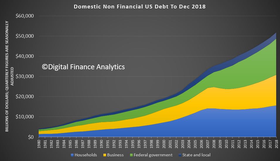
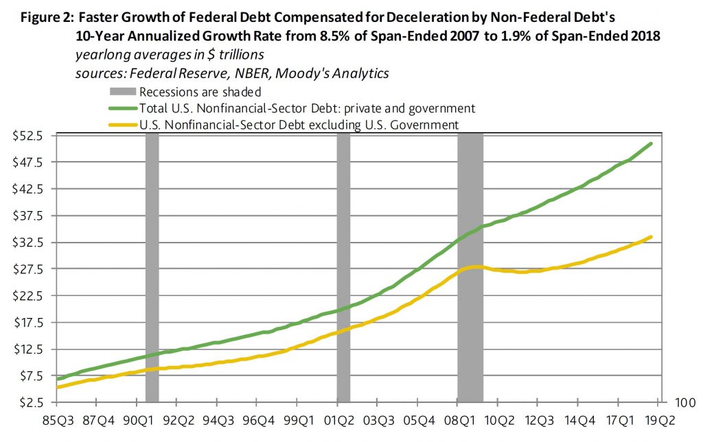
Moody’s says that US debt continues to rise (with strongest growth in the public sector) and a powerful enough external shock could force U.S. benchmark interest rates up to levels that shrink business activity considerably.
The latest version of the Federal Reserve’s “Financial Accounts of the United States” was released on March 7. As of 2018’s final quarter, the total outstandings of private and public nonfinancial-sector debt grew by 5.1% year-to-year to a record high $51.796 trillion. The year growth rate of the broadest estimate of U.S. nonfinancial-sector debt has slowed from second-quarter 2018’s current cycle high of 5.6%. Since the end of the Great Recession, the 3.9% average annualized rise by nonfinancial-sector debt has slightly outpaced nominal GDP’s accompanying 3.7% average annual increase.
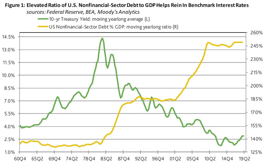
By contrast, during 2002-2007’s upturn, the 8.1% average annualized advance by nonfinancial-sector debt was much faster than nominal GDP’s comparably measured growth rate of 5.3%. As a result, the moving yearlong ratio of total nonfinancial-sector debt to GDP climbed from the 197% of 2001’s final quarter to the 225% of 2007’s final quarter. Because of the current recovery’s much slower growth of debt vis-a-vis GDP, debt barely rose from second-quarter 2009’s 243% to fourth-quarter 2018’s 249% of GDP.
Today’s near record high ratio of nonfinancial-sector debt to GDP limits the upside for benchmark interest rates. Just as highly leveraged businesses exhibit a more pronounced sensitivity to higher benchmark interest rates, highly leveraged economies are likely to slow more quickly in response to an increase by benchmark rates. Relatively low interest rates do much to lessen the burden implicit to a comparatively high ratio of debt to GDP.
Nevertheless, a powerful enough external shock could force U.S. benchmark interest rates up to levels that shrink business activity considerably. Under this scenario the Fed would be compelled to hike rates in defense of the dollar exchange rate despite how a deterioration of domestic business conditions requires lower rates.
The federal government has dominated the growth of total nonfinancial-sector debt during the current business cycle upturn. In terms of moving yearlong averages, U.S. government debt’s 9.3% average annualized surge has well outrun the accompanying 2.2% growth rate for the sum of private and state and local government nonfinancial-sector debt.
Regarding 2018’s final quarter, the outstandings of U.S. government debt advanced by 7.6% annually to $217.865 trillion. By comparison, household-sector debt rose by 3.1% to $15.628 trillion, nonfinancial corporate debt increased by 6.5% to $9.759 trillion, unincorporated business debt grew by 4.9% to $5.485 trillion, while state and local government debt shrank by 1.7% to $3.060 trillion. Thus, fourth quarter 2081’s U.S. nonfinancial-sector debt excluding the obligations of the federal government grew by a modest 3.9% annually. Over the past 10-years, the faster growth of federal government debt compensated for the sluggish debt growth of non-federal borrowers.
I will talk about how climate change affects the objectives of monetary policy and some of the challenges that arise in thinking about climate change.
Finally, I will also briefly discuss how climate change affects financial stability.
Let me start by highlighting a few of the dimensions that we need to consider:
We need to think in terms of trend rather than cycles in the weather. Droughts have
generally been regarded (at least economically) as cyclical events that recur every so
often. In contrast, climate change is a trend change. The impact of a trend is
ongoing, whereas a cycle is temporary.
We need to reassess the frequency of climate events. In addition, we need to reassess our
assumptions about the severity and longevity of the climatic events. For example, the
insurance industry has recognised that the frequency and severity of tropical cyclones (and
hurricanes in the Northern Hemisphere) has changed. This has caused the insurance sector to
reprice how they insure (and re-insure) against such events.
We need to think about how the economy is currently adapting and how it will adapt both to
the trend change in climate and the transition required to contain climate change. The
time-frame for both the impact of climate change and the adaptation of the economy to it is
very pertinent here. The transition path to a less carbon-intensive world is clearly quite
different depending on whether it is managed as a gradual process or is abrupt. The trend
changes aren’t likely to be smooth. There is likely to be volatility around the trend,
with the potential for damaging outcomes from spikes above the trend.
Both the physical impact of climate change and the transition are likely to have first-order
economic effects.
Climate Change, Economic Models and Monetary Policy
The economics profession has examined the effects of climate change at least since Nobel Prize
winner William Nordhaus in 1977. Since then, it has become an area of considerably more active
research in the profession.[4]
There has been a large body of research around the appropriate design of policies to address
climate change (such as the design of carbon pricing mechanisms), but not that much in terms of
what it might imply for macroeconomic policies, with one notable exception being the work of
Warwick McKibbin and co-authors.[5]
How does climate affect monetary policy? Monetary policy’s objectives in Australia are full
employment/output and inflation. Hence the effect of climate on these variables is an
appropriate way to consider the effect of climate change on the economy and the implications for
monetary policy. The economy is changing all the time in response to a large number of forces.
Monetary policy is always having to analyse and assess these forces and their impact on the
economy. But few of these forces have the scale, persistence and systemic risk of climate
change.
A longstanding way of thinking about monetary policy and economic management is in terms of
demand and supply shocks.[6]
A positive demand shock increases output and increases prices. The monetary policy response to a
positive demand shock is straightforward: tighten policy. Climate events have been good examples
of supply shocks. Indeed, droughts are often the textbook example used to illustrate a supply
shock. A negative supply shock reduces output but increases prices. That is a more complicated
monetary policy challenge because the two parts of the RBA’s dual mandate, output and
inflation, are moving in opposite directions. Historically, the monetary policy response has
been to look through the impact on prices, on the presumption that the impact is temporary. The
banana price episode in 2011 after Cyclone Yasi is a good example of this. The spike in banana
prices and inflation was temporary, although quite substantial. It boosted inflation by 0.7
percentage points. The Reserve Bank looked through the effect of the banana price rise on
inflation. After the banana crop returned to normal, prices settled down and inflation returned
to its previous rate.
The response to such a shock is relatively straightforward if the climate events are temporary
and discrete: droughts are assumed to end; the destruction of the banana crop or the closure of
the iron ore port because of a cyclone is temporary; things return to where they were before the
climate event. That said, the output that is lost is generally lost forever. It is not made up
again later, but rather output returns to its former level.
The recent IPCC report documents that climate change is a trend rather than cyclical, which makes the assessment much more complicated. What if droughts are more frequent, or cyclones happen more often? The supply shock is no longer temporary but close to permanent. That situation is more challenging to assess and respond to.
Climate Change and Financial Stability
Having talked about the macroeconomic impact of climate change and how that might affect monetary
policy, I will briefly discuss climate through the lens of financial stability implications.[10] Financial
stability is also a core part of the Reserve Bank’s mandate. Challenges for financial
stability may arise from both physical and transition risks of climate change. For example,
insurers may face large, unanticipated payouts because of climate change-related property damage
and business losses. In some cases businesses and households could lose access to insurance.
Companies that generate significant pollution might face reputational damage or legal liability
from their activities, and changes to regulation could cause previously valuable assets to
become uneconomic. All of these consequences could precipitate sharp adjustments in asset
prices, which would have consequences for financial stability.
The reason that I will only cover the implications of climate change for financial stability only
briefly today is that it has been very eloquently discussed by Geoff Summerhayes (APRA) and John
Price (ASIC) including at this forum over the past two years.[11] I would very much
endorse the points that Geoff and John have made. Geoff stresses the need for businesses,
including those in the financial sector to implement the recommendations of the Task Force for
Climate-related Financial Disclosures (TCFD).[12]
I strongly endorse this point. We have seen progress on this front in recent years, but there is
more to be done. Financial stability will be better served by an orderly transition rather than
an abrupt disorderly one.
One area that Geoff highlighted in a recent speech is that there is a data gap which needs to be
addressed:[13] ‘The
challenge governments, regulators and financial institutions face in responding to the
wide-ranging impacts of climate change is to make sound decisions in the face of uncertainty
about how these risks will play out.’ In that regard, Geoff mentions one challenge that I
spoke about earlier in the context of monetary policy. Namely, taking the climate modelling and
mapping that into our macroeconomic models. For businesses and financial markets, that challenge
is understanding the climate modelling and conducting the scenario analysis to determine the
potential impact on their business and investments.
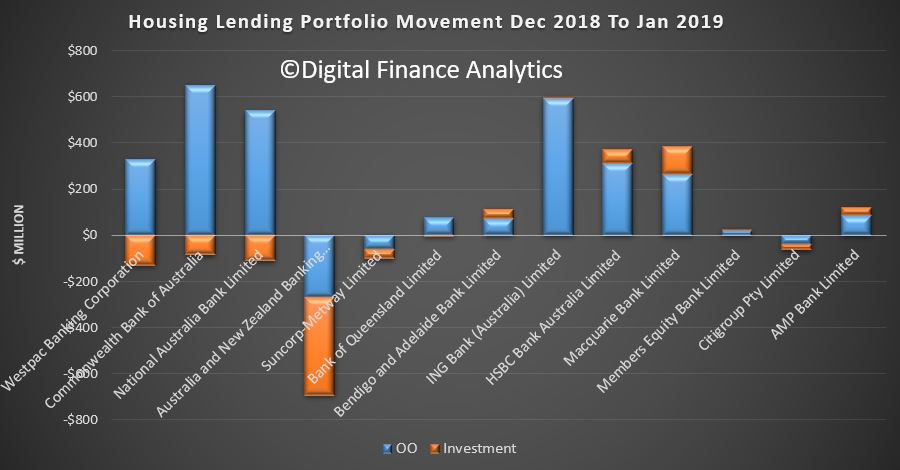
The value of new lending commitments to households fell 2.4 per cent in January 2019, seasonally adjusted, according to the latest Australian Bureau of Statistics (ABS) figures on new lending to households and businesses.
The fall in lending to households in January follows a revised 3.6 per cent monthly fall in December 2018.
ABS Chief Economist, Bruce Hockman said: “Weaker lending for dwellings (-2.1 per cent) again drove much of the overall fall in lending to households, with further falls in lending for investment dwellings (-4.1 per cent) and for owner occupier dwellings (-1.3 per cent) in January.”
“Reflecting the impact of both supply and demand side factors, new lending for dwellings is down over 20 per cent from January 2018, the largest through the year decline since late 2008.”, he said.
This weaker lending activity was evident across the states and territories in January, with new lending for investment dwellings down in all states and territories. Only Queensland and the Northern Territory recorded rises in lending for owner occupier dwellings.
While there was also a fall in the number of loans to owner occupier first home buyers (-0.3 per cent) in January, this was more stable than the 3.2% fall in the number of loans to owner occupier non-first home buyers.
Lending to households for personal finance (up 1.2 per cent) was the only household lending category to record a rise in January, however new lending is down 16.0 per cent compared to January 2018, seasonally adjusted. The value of lending to households for refinancing fell 3.4 per cent.
In trend terms, the value of new lending commitments to businesses fell 1.3 per cent in January, but is up 2.5 per cent from January 2018.
More evidence of the peeling back of US bank disclosure, which may reduce the incentive for bank managements to continually improve their capital and risk management processes.
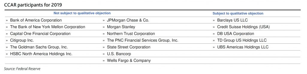
On 6 March, Moody’s says the US Federal Reserve Board (Fed) announced the elimination of the qualitative objection in its 2019 Comprehensive Capital Analysis and Review (CCAR) for most stress test participants. Only five banks, all US subsidiaries of foreign banks, will remain subject to qualitative objection in the current stress tests cycle. In the past, the Fed has used the qualitative objection to address deficiencies in banks’ capital-planning process. Its elimination is credit negative because it reduces public transparency around the quality of banks’ internal capital and risk management processes.
Under the revised rules, a bank must participate in four CCAR cycles before it qualifies for exemption from a potential qualitative objection in future years. If a firm receives a qualitative objection in its fourth year, it will remain subject to a possible qualitative objection until it passes. For most of the five firms still subject to the qualitative objection, their fourth year will be the 2020 CCAR cycle. In total, 18 firms are subject to this year’s CCAR exercise, with five of them subject to a possible qualitative objection.
All five firms subject to the qualitative assessment in 2019 are foreign-owned intermediate holding companies (IHCs), most of which were first subject to the Fed stress tests on a confidential basis in 2017. If the IHC has a bank holding company subsidiary that was subject to CCAR before the formation of the IHC, then the IHC is not considered the same firm for the purpose of the four-year test.
The Fed noted that since CCAR was implemented in 2011, most firms have significantly improved their risk management and capital planning process. Going forward, its capital-planning assessments will be through the regular supervisory process. The Fed highlighted as an example the new rating system for large financial institutions, which will assign component ratings of a firm’s capital planning and positions. However, these ratings will be confidential supervisory information and unavailable to the public unless the deficiencies are so severe that they warrant formal enforcement action. The new process replaces an independent comparative assessment.
The lack of public disclosure may also reduce the incentive for bank managements to continually improve their capital and risk management processes, which the CCAR qualitative review encouraged.
As previously announced, 17 large and non-complex bank holding companies, generally with $100-$250 billion of consolidated assets, will not be subject to CCAR in 2019 because of the Economic Growth, Regulatory Relief, and Consumer Protection Act (the EGRRCPA), which became law in May 2018. They will next participate in 2020. Most of these banks were removed from the qualitative objection in 2017 and the Fed will only object to their capital plans if they fail to meet one of the minimum capital ratios under the stress scenarios on quantitative grounds.
The Fed’s announcement was incorporated with its release of instructions for the 2019 CCAR cycle. The Fed also provided information on allowable capital distributions for those firms whose CCAR cycle was extended to 2020. For those banks, the Fed published letters that address each bank’s individual 2019 capital plans. The Fed pre-authorized the firms to distribute, net of any issuance of capital, up to the sum of:
The additional capital the firm could have distributed in CCAR 2018 and remained above the minimum requirements; plus
Capital accretion (change in capital ratios since CCAR 2018); plus
its already approved capital distributions for first-quarter 2019 and second-quarter 2019; minus
its actual distributions for first-quarter 2019 and planned distribution for second-quarter 2019
This plan is also credit negative because it permits capital distributions based on last year’s results, which incorporated a modestly less stringent severely adverse scenario than the 2019 stress test, and it also fails to incorporate any interim changes in the banks’ risk profiles. If any of the 17 banks wants to distribute more than its maximum pre-authorized amount, it may submit a capital plan to the Fed by 5 April 2019 and will be subject to the 2019 CCAR supervisory stress test.
Australia’s major banks will continue to face heightened regulatory scrutiny following recent public inquiries, including the Royal Commission, that identified shortcomings in conduct, governance and compliance, and will all be engaged in remediation that could distract management from day-to-day business, says Fitch Ratings. These challenges come amid other near-term pressures on earnings from a generally tougher operating environment.
The four major banks –
ANZ, CBA, NAB, Westpac – have large market shares across most products
in Australia and New Zealand, which support strong earnings and balance
sheets and help moderate risk appetite compared with many international
peers. However, it may be difficult for the banks to exercise these
advantages fully in an environment of increased public and regulatory
scrutiny, and pressure to increase their focus on customers rather than
shareholders.
In the longer term, there is a risk that the
findings of the inquiries may erode the market position of the four
major banks, either by reducing management focus on revenue growth or
through reputational damage – of which there is so far little evidence.
CBA
and NAB were found to have the most significant weaknesses in their
operational and compliance risk frameworks, and therefore face larger
risks from the remediation process. This is reflected in the Negative
Outlooks Fitch has assigned to these banks’ Long-Term Issuer Default
Ratings. Shortcomings that allowed misconduct issues to arise were
particularly evident at CBA, which is the only bank that will go through
to a formal remediation process and face increased capital
requirements.
Addressing conduct, culture and governance
problems should improve the soundness of the system in the longer term,
but will exacerbate banks’ short-term challenges. Fitch maintains a
negative outlook on the sector as earnings are likely to remain under
pressure in 2019 due to slower loan growth, especially in the
residential-mortgage segment, falling net interest margins, rising
wholesale funding costs, and increasing impairment charges, albeit from a
low level.
The main downside risks to bank performance continue
to stem from the housing market, where prices continue to decline after
large increases up to mid-2017. A sharp drop may result in negative
wealth effects for consumers and could undermine banks’ asset quality.
However, our central scenario is that house prices will fall by only
around 5% in 2019, which would represent a gradual easing of housing
market risks. Moreover, regulatory intervention in the mortgage sector,
including more stringent underwriting measures, has helped to reduce
risks in newer vintages of loans, and should make the major banks more
resilient to any downturn.
Weeks after posting a 97% drop in profits, AMP has announced changes to its home loan offerings, via Australian Broker.
In the next few days, AMP Bank plans to decrease a range of fixed rate loan options as well as increase variable rates.
“We have held off passing this cost on to existing customers for as
long as we can. We are managing our loan portfolio in a very active
market and decisions on rates are never taken lightly,” said AMP chief
executive Sally Bruce.
When the bank shared its financial results in mid-February, it
attributed its 2018 earnings being less than the year before to several
factors, including higher cash outflows and the ongoing impact of the
royal commission.
Now, variable lending rates for new and existing owner occupiers and investors will increase by 0.15% p.a.
“The change in variable rates is driven by an increase in costs,” said Bruce.
The bank also announced two new fixed lending offers: the three-year
package investment P&I at 3.99% per year, and the five-year package
owner occupied P&I at 4.05%.
AMP clarified that the two-year fixed rate of 3.75% for owner
occupied principal and interest customers will continue to be offered.
The rate changes go into effect on 8 March for new business and 11 March for existing business.
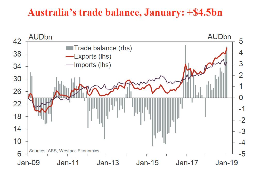
The ABS released the latest trade data to end January 2019. The surplus jumped to $4.5bn which is the second highest on record. The largest was $4.7bn surplus in December 2016.
Westpac highlighted that the January outcome was a $0.8bn improvement on December and exceeded expectations (market median $2.75bn and Westpac $3.1bn).
Imports did rebound in the month, +3.3%, following a 5.5% fall last month (vs a forecast +4%).
Exports were much stronger than anticipated, increasing by 5.0%, up $1.9bn (vs a forecast +2.2%).
Export strength was largely centred on a sharp rebound in gold off a low base, up 174% (Westpac expected a 75% rebound).
In dollar terms, gold accounted for $1.4bn of the $1.9bn increase in total exports in the month.
Coal exports rose 6%, following a couple of softer months, and metal ores increased by 3.4%, boosted by the higher iron ore price. But rural exports have been more resilient over the past couple of months – however the drought in NSW and surrounds remains a considerable headwind.
Metal ores and coal both advanced in January, up a combined $0.6bn.
The trade surplus widened in 2018 and in to 2019 on higher export earnings, boosted by rising commodity prices.
Notably, commodity prices have surprised to the high side in part due to supply disruptions having an amplified impact in a market where supply and demand are in relatively tight balance.
The $4.5bn surplus for January compares with a Q4 monthly average of $2.8bn.
The surplus for Q1 as a whole is expected to be a material improvement on that in Q4, with export volumes forecast to rise (following a disappointing second half of 2018) and on a likely further increase in the terms of trade.