Property Market – Page 194 – Digital Finance Analytics (DFA) Blog

The Dynamics of US Mortgage Debt in Default

Research from the USA highlights the fact that when house prices fall, and household debt is high, the rise in defaults is more correlated to the number of households falling behind in their mortgage payments that the debts of those already in default.

From St. Louis Fed Research

The large decrease in US house prices between 2006 and 2011 led to a dramatic increase in mortgage debt defaults. Since then, the share of mortgage debt in default has decreased significantly and is now close to the pre-2006 level. In this essay, we argue that these fluctuations are predominantly the consequence of changes in the number of households falling behind in their mortgage payments (the extensive margin) and not changes in the amount of debt of those in default (the intensive margin). On average, the extensive margin accounts for 78 percent of the increase in the 2006-09 period and 93 percent of the decrease in the 2011-15 period. This information may be useful in designing prudential policies to mitigate mortgage default.

The analysis is performed using data from the Federal Reserve Bank of New York Consumer Credit Panel/Equifax. In our measure of default, we consider all households with mortgage payments 120 or more days late. Figure 1 shows the share of mortgage debt in default, which fluctuated between 0.7 percent and 1 percent in the 1999-2006 period and then jumped to 7.5 percent in 2009. The figure also shows the evolution of house prices, whose collapse coincided with increasing mortgage defaults. In a recent article, Hatchondo, Martinez, and Sánchez (2015) show how these two series are related: A rapid decrease in house prices causes a sharp increase in mortgage defaults because more households find themselves with negative home equity (“under water”), and some of these households find it beneficial to default after a negative shock to income (i.e., unemployment).

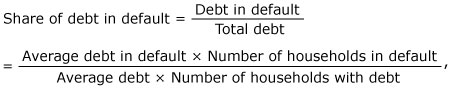
We decompose the changes in the share of debt in default into changes in four different components: average debt in default, number of households in default, average debt, and number of households with debt. Basically, since

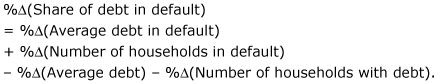
we can compute the percentage change (%∆) in the share of debt in default as follows:

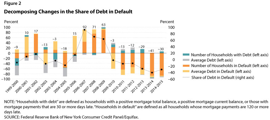
Figure 2 shows the results of the decomposition by year; the four colors in each column represent the changes in the four components. The percentage value (shown on the left vertical axis) illustrates the change in the share of debt in default generated by the changes in a particular component. According to the previous equations, the summation of changes in the four components equals the changes in the share of debt in default (represented by the values for the black dots as shown on the right axis). For example, the black dot for 2006-07 has a value of 92, which indicates that the share of debt in default increased by 92 percent in that time period.

There are three interesting findings. First, and most importantly, we find that fluctuations in the number of households in default accounted for most of the fluctuations in the share of debt in default (shown by the size of the orange part of the bars in Figure 2). The share of households in default was very large not only for the years when defaults were increasing (2006 to 2009), but also for the subsequent years when the share of debt in default decreased slowly but steadily. The changes in the number of households in default confirm our earlier claim that the drastic decline in house prices between 2006 and 2009 caused negative home equity for more households. For some of these households a negative income shock triggered default, thus leading to the sharp increase in mortgage debt default. Another reason for this pattern is the delay in foreclosure proceedings that started during the Great Recession. Chan et al. (2015) show that borrowers’ knowledge of a possible long delay between the formal notice of foreclosure and the actual foreclosure sale date affects the likelihood of default: Borrowers who anticipate a longer period of “free rent” have a greater incentive to default on their mortgages.

Second, our results indicate that from 2003 to 2007 the average amount of debt (the gray part of the bars in Figure 2) exerted downward pressure on the share of debt in default. That is, since the average amount of debt was increasing, if the other three components had not increased, the share of debt in default would have decreased.

Finally, we find that the average amount of debt in default (the yellow part of the bars in Figure 2) was important in the 2006-08 period. This finding indicates that part of the increase in the share of debt in default during that period was actually due to an increase in the amount of the debt of households in default. This increase is in line with the fact that the decline in house prices affected households with larger debt (not necessarily subprime loans) that were not falling into default before 2006. When house prices plummeted in 2006, more households from this group defaulted. Later in the recession, the importance of the average amount of debt was overtaken by the number of households in default as more and more households with similar characteristics chose to default.

To summarize, the rapid increases in mortgage debt in default between 2006 and 2011 captured the attention of the public, policymakers, and researchers. It is important to understand the main forces driving the default increase, especially in designing prudential policies that minimize mortgage default such as those analyzed by Hatchondo, Martinez, and Sánchez (2015). The decomposition exercise in this essay suggests that the evolution of the share of mortgage debt in default can be accounted for mostly by changes in the number of households in default rather than changes in the overall amount of mortgage debt and the number of households with mortgages. Changes in the amount of debt in default also played a nonnegligible role, especially during the pre-crisis to early crisis periods.

OO Housing Finance Bounces Back – Refinance Anyone?

The latest ABS data to December 2015 shows that in the month, trend owner occupied lending grew 1.3%, seasonally adjusted, with $21.3 bn of loans being written. Construction loans grew 1.4% ($1.9 bn), purchase of new dwellings grew 1.7% ($1.3bn) and purchase of established dwellings by 1.28% ($18.75bn). Refinance continued to grow, with 33% of loans written in the month churned, up 2.3% to $7.29bn. Overall owner occupied lending, net of refinance grew just 0.8%.

Looking at state trends, VIC led the way, up 1.5%, QLD at 1%, NSW at 0.7%, SA 0.6%, and WA down 0.3%. But startlingly, TAS reported a rise of 1.8% and NT a rise of 1.4%. The ACT was 1.6% higher. So, WA apart, owner occupied lending grew in every state.

Total finance, including investment loans grew by just 0.025%, investment loans fell 2.36% to 11.4 bn. We see the clear focus of lending is to owner occupied borrowers, and a massive focus on churning loans. We also see a significant rise in the number of fixed rate deals, as households lock in low rates, with the number of deals up 17.2%, whilst secured revolving loans fell 9.8%. This reflects the cheap loan special offers which are currently in the market.

First time buyer OO loans grew in December, with a rise of 4.6% on the previous month to make up 15.1% of new loans. This is faster than for non-first time buyer loans, here the number of loans grew 3.1%. The average loan size fell a little in the month, reflecting tighter lending criteria. This is original data, not trend smoothed.

Overlaying first time investors, from our surveys, overall first time buyers were more active, still wanting to get on the property ladder one way or the other. FTB investors grew by 6.5% in the month, after a couple of slow months before. Overall, about 14,000 first time buyer deals were done.

Owner Occupied Demand Stronger – ME Bank

ME’s latest Property Buying Intentions Report indicates demand for residential property may remain strong over the next 12 months despite prudential changes and tightening of lending criteria for some home buyers. The Report shows a big jump in demand for property by owner occupiers potentially offsetting falling demand by investors, while buyers continue to outnumber sellers.

According to the Report:

In the six months to December 2015, the proportion of Australians intending to buy a property/home fell 1 point to 17%, matched by a correspondingly small fall in the proportion intending to sell a property/home (down 1 point to 7%). Buyers continue to outnumber sellers by more than two-to-one.
Over the same six month period and among those actively looking to buy and/or sell property during 2016, there was a 5 point increase to 50% in the proportion looking to buy a home to live in (owner occupier buyers) offsetting a 5 point fall to 33% in the proportion looking to buy an investment property (investor buyers).
Also among those active in the property market, planned sales by home owners remained unchanged over the six months to December at 26%, while there were fewer intended sellers of investment properties (down 5 points to 8%).

ME Treasurer, John Caelli, said notwithstanding other factors, the findings indicate property demand pressures from buyers may remain strong over the next 12 months. “While recent tightening in bank prudential regulations and lending criteria have reduced the proportion of investor buyers, overall demand for property may remain strong due to increased demand by owner occupier buyers. “Demand expectations from buyers may also remain strong due to unmet demand from owner occupiers supported by continued low borrowing costs and recent improvements in the labour market.”

Other findings

23% of Gen Y are saving to buy a property to live in and 25% intend to buy a property to live in in the next 12 months, the most of any age group.
10% of Gen X are saving to buy an investment property and 8% intend to buy an investment property in the next 12 months, the most of any age group.
The proportion of first home buyers has increased slightly to 22% in the six months to December 2015, up 1 point.
Of those actively looking to buy or sell a home to live in in the 12 months, 19% are downsizers, 22% are upgraders and 59% are looking for property with a similar price point.

About the House Buying Intentions Report

ME commissioned DBM Consultants to conduct an online survey of approximately 1,500 Australians aged 18 years and older who do not work in the market research or public relations industries. The population sample was weighted according to ABS statistics on household composition, age, state and employment status to ensure that the results reflected Australian households.

Australian Housing Unaffordable – Demographia

The 2016 Demographia survey (the 12th edition) is out using data from Q3 2015. Once again Australians are shown to be exposed to highly unafforable housing, with all the downstream economic consequences which follow. Policy, regulation, and vision have all failed us. Whilst inflated prices bloat banks’ balance sheets thanks to massive lending for housing, the economic outcomes are disastrous. The resulting stagnation or even decline in household discretionary incomes is at least as much a threat to prosperity and job creation as the limited gross income gains.

” Australia had 33 severely unaffordable markets, followed by the United States with 29 and the United Kingdom with 17. New Zealand and Canada each had six severely unaffordable markets, while China’s one market (Hong Kong) was also severely unaffordable.”

The survey covers 367 metropolitan markets in nine countries (Australia, Canada, China, Ireland, Japan, New Zealand, Singapore, the United Kingdom and the United States). A total of 87 major metropolitan markets — with more than 1,000,000 population — are included, including five megacities (Tokyo-Yokohama, New York, Osaka-Kobe-Kyoto, Los Angeles, and London).

The Demographia International Housing Affordability Survey rates middle-income housing affordability using the Median Multiple.” The Median Multiple is widely used for evaluating urban markets, and has been recommended by the World Bank and the United Nations and is used by the Joint Center for Housing Studies, Harvard University. The Median Multiple and other similar price-to-income multiples (housing affordability multiples) are used to compare housing affordability between markets by the Organization for Economic Cooperation and Development, the International Monetary Fund, The Economist, and other organizations.

Demographia uses the following housing affordability ratings:

Severely Unaffordable 5.1 & Over
Seriously Unaffordable 4.1 to 5.0
Moderately Unaffordable 3.1 to 4.0
Affordable 3.0 & Under

Hong Kong’s Median Multiple of 19.0 was the highest recorded (least affordable) in the 12 years of the Demographia International Housing Affordability Survey. Sydney was the second least affordable major market, with a Median Multiple of 12.2. Sydney’s increase of 2.4 points from its 9.8 Median Multiple in 2014 is the largest year-to-year deterioration ever indicated in the 12 years of the Demographia International Housing Affordability Survey. It is also highest Median Multiple outside Hong Kong in the history of the Survey, exceeding the extremes experienced on the US West Coast during the housing bubble of the last decade. Vancouver was the third least affordable major market, with a Median Multiple of 10.8. Auckland, Melbourne and San Jose all had Median Multiples of 9.7. They were followed by San Francisco at 9.4, and London (Greater London Authority), at 8.5. Two other markets had Median Multiples of 8.0 or above, including San Diego and Los Angeles, both at 8.1.

Virtually all governments consider household economic issues as a top priority, especially increasing the standard of living and reducing or eradicating poverty. Yet economic growth has been laggard, and discretionary income trends are even more concerning. Housing costs, which represent the largest household expenditure category, have been rising much faster than incomes. The resulting stagnation or even decline in household discretionary incomes is at least as much a threat to prosperity and job creation as the limited gross income gains.

The largest losses in housing affordability have been associated with urban containment policy. Severely unaffordable housing (Median Multiple of 5.1 or higher) has occurred only in major metropolitan areas that have strong land use policy, especially urban containment boundaries and variations thereof. Corrective measures that could halt or reverse losses in housing affordability from urban containment policy have either been absent or not been implemented. As a result, urban containment policy has been a profound policy failure, as house prices have doubled and tripled relative to incomes in many metropolitan areas.

In the introduction, Senator Bob Day says:

For more than 100 years the average Australian family was able to buy its first home on one wage. The median house price was around three times the median income allowing young home buyers easy entry into the housing market As can be seen from the graph below (“ Real Home Price Index”), the median house price has increased, in real terms, by more than 300% – from an average index of 100 between 1900 and 2000 to an index over 300 by the year 2008.

Relative to incomes, house prices have increased from three times median income to more than nine times income. That’s $600,000 they are not able to spend on other things – clothes, cars, furniture, appliances, travel, movies, restaurants, the theatre, children’s education, charities and many other discretionary purchase options.

It is a similar story in the UK, US, Canada, New Zealand, Ireland and Japan.

The economic consequences of this change have been devastating. The capital structure of these countries’ economies have been distorted to the tune of hundreds of billions of dollars and for those on middle and low incomes the prospect of ever becoming homeowners has now all but vanished. Housing starts are below what they should be and so have all the jobs associated with them – civil construction, house construction, transport, appliances, soft furnishings, you name it. Not to mention billions of dollars in lost taxes and other housing-related revenue to the nation state.

The distortion in the housing market, this misallocation of resources resulting from the supply-demand imbalance is enormous by any measure and affects every other area of a country’s economy. New home owners pay a much higher percentage of their income on house payments than they should. Similarly, renters are paying increased rental costs reflective of the higher capital and financing costs in turn paid by landlords.

Economies have been distorted and getting them back into alignment is going to take some time. But it is a realignment that is necessary. A terrible mistake was made and it needs to be corrected.

Foreign Investor Forced Property Sales Announced

From Mortgage Professional Australia.

The Federal Government’s crackdown on the illegal ownership of Australian real estate has continued, with it announcing the forced sale of eight residential properties.

According to the government, the eight properties, valued between $200,000 and $5 million, bring the total number of forced sales since the Coalition formed government to 27.

The eight properties in question were owned by investors from five different countries.

“The individuals involved come from a range of countries – Canada, China, India, Malaysia and the United States of America,” Federal Treasurer Scott Morrison said.

“The foreign investors either purchased established residential property without Foreign Investment Review Board approval, or had approval but their circumstances changed meaning they were breaking the rules,” Morrison said.

Morrison said the discovery of the illegal ownership of the eight properties was thanks to new powers granted to the Australian Taxation Office (ATO).

“The Government’s transfer of responsibility to the ATO for compliance has enabled more active investigations and actions targeting illegitimate purchases,” he said.

“Since this transfer in May, over 1,500 matters have been referred for investigation. Through information provided by the public, together with the ATO’s own enquiries, over 800 cases remain under active investigation.”