Melbourne is officially Australia’s fastest growing capital city, according to data released today by the Australian Bureau of Statistics (ABS).
Melbourne’s population grew by 2.1 per cent in 2014-15, down slightly from 2.2 per cent last year, but still higher than the next-fastest growing capital, Darwin (1.9 per cent).
Perth, which has been one of the fastest-growing capital cities since the mid-2000s, grew by 1.6 per cent in 2014-15 (down from 1.9 per cent last year) and now sits equal fourth with Brisbane, behind Sydney (1.7 per cent).
“Although Perth’s growth slowed to its lowest rate since 2004-05, it was not the only city to experience weaker growth,” said ABS Director of Demography Beidar Cho.
“Of all the capitals, only Hobart (0.8 per cent), Canberra (1.4 per cent) and Darwin (1.9 per cent) grew faster in 2014-15 than in the previous year”.
Australia’s capital cities accounted for the vast majority (83 per cent) of the nation’s total population growth in 2014-15, with most growth occurring in outer suburban and inner city areas.
The fastest growing areas in each state and territory were Cobbitty – Leppington (New South Wales), Cranbourne East (Victoria), Pimpama (Queensland), Munno Para West – Angle Vale (South Australia), North Coogee (Western Australia), Rokeby (Tasmania), Palmerston – South (Northern Territory), and ACT – South West (Australian Capital Territory).
New South Wales – Sydney is well on target to becoming the first Australian capital city to reach 5 million people, growing by 83,300 in 2014-15 to hit 4.92 million.
Victoria – Melbourne had both the largest (91,600) and fastest (2.1 per cent) population increase of all Australian capital cities in 2014-15.
Queensland – Brisbane’s population may be increasing at its slowest rate for over a decade, but Queensland has some of the largest-growing regional areas in the nation.
South Australia – Adelaide’s outer suburbs may be experiencing the largest population increases, but some of the city’s fastest growth is occurring in its inner areas.
Western Australia – Perth’s growth has slowed to its lowest rate for a decade, increasing by 1.6 per cent in 2014-15 compared with 1.9 per cent in 2013-14.
Tasmania – Although growing at the slowest rate of all capital cities (0.8 per cent in 2014-15), Hobart is the only Australian capital to record an increasing rate of population growth in each of the last three years.
Northern Territory – Darwin remains one of the fastest-growing capital cities in Australia, increasing by 1.9 per cent in 2014-15, second only to Melbourne (2.1 per cent).
Australian Capital Territory – The newly-developed suburbs of Canberra’s Molonglo Valley are the fastest-growing areas in Australia. The population of ACT – South West, which includes the new suburbs of Wright and Coombs, grew by 127 per cent in 2014-15.
Category: Social Trends
Four reasons payday lending will still flourish despite Nimble’s $1.5m penalty
The payday lending sector is under scrutiny again after the Australian Securities and Investment Commission’s investigation into Nimble.
After failing to meet responsible lending obligations, Nimble must refund more than 7,000 customers, at a cost of more than A$1.5 million. Aside from the refunds, Nimble must also pay A$50,000 to Financial Counselling Australia. Are these penalties enough to change the practices of Nimble and similar lenders?
It’s very unlikely, given these refunds represent a very small proportion of Nimble’s small loan business – 1.2% of its approximately 600,000 loans over two years (1 July 2013 – 22 July 2015).
The National Consumer Credit Protection Act 2009 and small amount lending provisions play a critical role in protecting vulnerable consumers. Credit licensees, for example, are required to “take reasonable steps to verify the consumer’s financial situation” and the suitability of the credit product. That means a consumer who is unlikely to be able to afford to repay a loan should be deemed “unsuitable”.
The problem is, regulation is just one piece of a complex puzzle in protecting consumers.
- It’s going to be difficult for the regulator to keep pace with a booming supply.Nimble ranked 55th in the BRW Fast 100 2014 list with revenue of almost A$37 million and growth of 63%. In just six months in 2014, Cash Converters’ online lending increased by 42% to A$44.6 million. And in February 2016, Money3 reported a A$7 million increase in revenue after purchasing the online lender Cash Train.
- Consumers need to have high levels of financial literacy to identify and access appropriate and affordable financial products and services.The National Financial Literacy Strategy, Money Smart and Financial Counselling Australia, among other providers and initiatives, aim to improve the financial literacy of Australians, but as a country we still have significant progress to make. According to the Financial Literacy Around the World report, 36% of adults in Australia are not financially literate.
- The demand for small loans is high and yet there are insufficient supply alternatives to payday lending in the market.The payday loan sector dominates supply. Other options, such as the Good Shepherd Microfinance No Interest Loan Scheme (NILS) or StepUP loans, are relatively small in scale. As we’ve noted previously, to seriously challenge the market, realistic alternatives must be available and be accessible, appropriate and affordable.
- Demand is not likely to decrease. People who face financial adversity but cannot access other credit alternatives will continue to seek out payday loans.ACOSS’s Poverty in Australia Report 2014 found that 2.5 million Australians live in poverty. Having access to credit alone is not going to help financially vulnerable Australians if they experience an economic shock and need to borrow money, but lack the economic capacity to meet their financial obligations.
Social capital can be an important resource in these situations. For example, having family or friends to reach out to. This can help when an unexpected bill, such as a fridge, washing machine or car repair, is beyond immediate financial means. Yet, according to the Australian Bureau of Statistics General Social Survey, more than one in eight (13.1%) people are unable to raise A$2,000 within a week for something important.
Coupled with regulation, these different puzzle pieces all play an important role in influencing the entire picture: regulators and regulation; the supply of accessible, affordable and appropriate financial products; the financial literacy and capacity of consumers; people’s economic circumstances; and people’s social capital.
Previous responses to financial vulnerability have often focused on financial inclusion (being able to access appropriate and affordable financial products and services), financial literacy (addressing knowledge and behaviour), providing emergency relief, or regulating the credit market. Dealing with these aspects in silos is insufficient to support vulnerable consumers.
A more holistic response is needed: one that puts the individual at the centre and understands and addresses people’s personal, economic and social contexts. At the same time, it must factor in the role of legislation, the market and technology.
The Turnbull government recently committed to “creat[ing] an environment for Australia’s FinTech sector where it can be internationally competitive”.
With more online lenders coming, it’s important we work towards strengthening people’s financial resilience.
Improving the financial resilience of the population, coupled with strong reinforced regulation, will help to protect financially vulnerable Australians from predatory lenders.
Authors: Kristy Muir, Associate Professor of Social Policy / Research Director, Centre for Social Impact, UNSW Australia; Fanny Salignac,
Research Fellow – Centre for Social Impact, UNSW Australia; Rebecca Reeve, Senior Research Fellow, Centre for Social Impact, UNSW Australia
The Transport Sector Shakedown Has Real Consequences
In less than a week (4 April 2016), transport costs could rise significantly, thanks to the Road Safety Remuneration Tribunal (RSRT) order which implements a minimum rate for contractor drivers through the Contractor Driver Minimum Payments Road Safety Remuneration Order. This sets a national minimum payments for contractor drivers in the road transport industry. A few key points about the order:
- You will not be allowed to trade as either a sole trader or partnership you must use a company.
- The company that owns the truck cannot be owned by either yourself, a family member or friend.
- Driver rates from the RSRT apply only to “owner operators” not ASX listed transport operators, so an OO will have to charge a lot more.
- Freight rates will have to go up at least 40% which will flow through to the entire economy.
- The Road Safety Remuneration Tribunal (RSRT) will be around for 3 years before undergoing a review.
Many are saying that if the changes to minimum rates proceed, it will price smaller operators out of the industry, though the Transport Workers Union (TWU) is a vocal supporter of the Order. It says an increase in minimum rates will make the industry safer, and that’s worth paying for.
However, according to Business Spectator, some 35,000 people, mostly men, drive their own long-haul trucks. They have borrowed around $15 billion from Australian banks and other financiers to fund their vehicles. Most of the loans are also secured on the family home.
So, consider the implications. First, the average cost of a truck is ~200k. The Personal Property Securities Register regime means that lenders would have the power to sell the asset at once – and if they cannot on-sell the vehicle, then its scrap value of ~$23 a tonne is the going rate. Then they can turn to the borrowers other assets. We could see a spate of forced home sales.
Second, the finance sector has dedicated resources servicing the truck finance and insurance sector, plus there is a network of dealers, repairers, accommodation providers, and other services which will be impacted as demand falls for their services.
Third, who will still be on the road to provide transport services – the big guys, of course. But will they want to provide the range of services currently available? Possibly not. So will there be significant transport disruption?
At very least, what was an invisible cost is certainly going to become visible, but we wonder if the knock-on effects have really be thought through.
Australians intend to work longer than ever before – ABS
Australians aged 45 years and over are intending to work longer than ever before, according to figures released by the Australian Bureau of Statistics (ABS) today.
In the survey conducted in 2014-15, 71 per cent of persons intended to retire at the age of 65 years or over, up from 66 per cent in last survey result of 2012-13 and 48 per cent in 2004-05.
“The survey found that 23 per cent of the persons aged 45 years and over are intending to retire at the age of 70 years or over compared with only eight per cent in 2004-05,” said Jennifer Humphrys from the ABS.
The average intended retirement age is 65 years (66 years for men and 65 years for women).
“The majority of Australians intend to retire between 65-69 years, but the results show that now over a quarter of males 45 years and over plan to work past 70 years.”
The survey commenced a few months after the government announced changes to the current qualification age for the Age Pension.
For those in the labour force who intended to retire, the most common factors influencing their decision were ‘financial security’ (40 per cent for men and 35 per cent for women) and ‘personal health or physical abilities’ (23 per cent for both men and women).
Just over half (53 per cent) reported their main expected source of personal income at retirement as ‘superannuation/annuity/allocated pension’.
“There were some differences reported by those who had already retired compared with those who intended to retire regarding their main (expected) source of personal income at retirement,” said Ms Humphrys.
“While 47 per cent of persons aged 45 years and over who had retired reported a ‘government pension or allowance’ as their main source of income at retirement, only 27 per cent of persons aged 45 years and over who were intending to retire indicated that this would be their main expected source of income at retirement.”
The survey also highlighted the importance of partner’s income as one of the main expected source of funds for meeting living costs at retirement.
“Although personal income was a common expected source for both men (81 per cent) and women (70 per cent), 13 per cent of women expected to rely on ‘partner’s income’ in contrast to only three per cent of men. However, while only seven per cent of those intending to retire were expected to rely on partner’s income, this was reported as the main source of funds for meeting living costs by 26 per cent of the retirees,” said Ms Humphrys.
More details are available in Retirement and Retirement Intentions, Australia (cat. no. 6238.0),
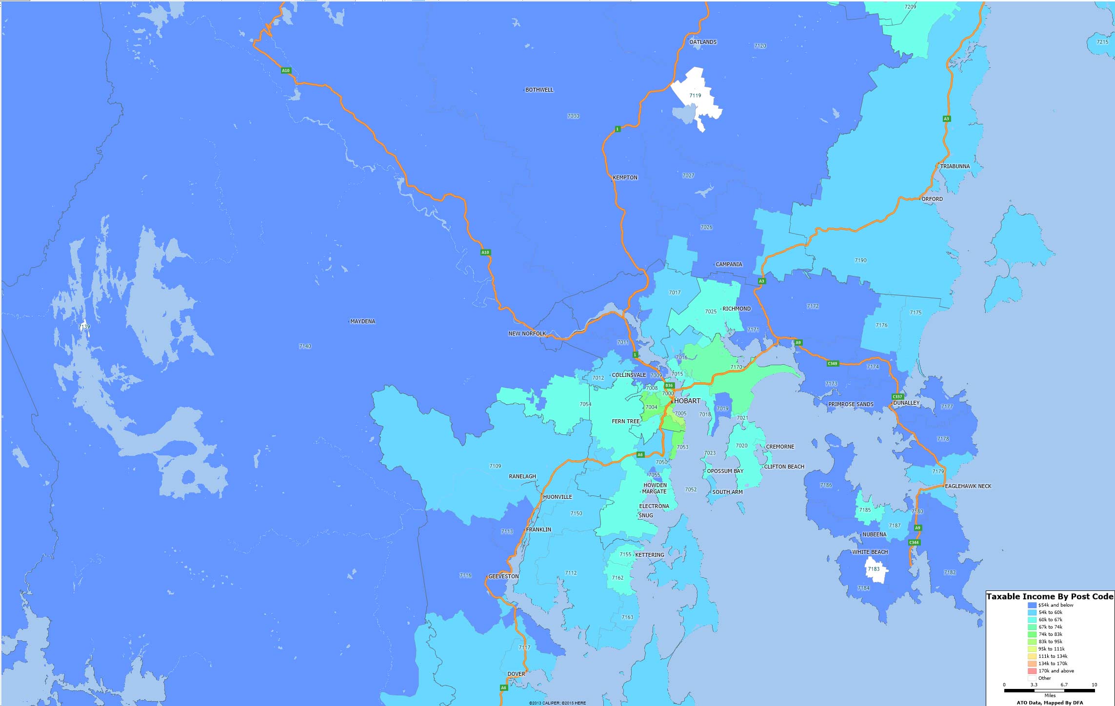
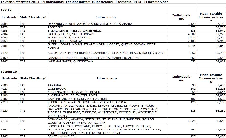
Hobart Region Taxable Income Heat Map 2014 and National Summary
Today we finish our series of taxable income heat maps, using data from the ATO, from 2013-2014, looking at Hobart. Then finally, we include a nationwide top ten summary.
 Here are the top and bottom 10 postcodes in the state.
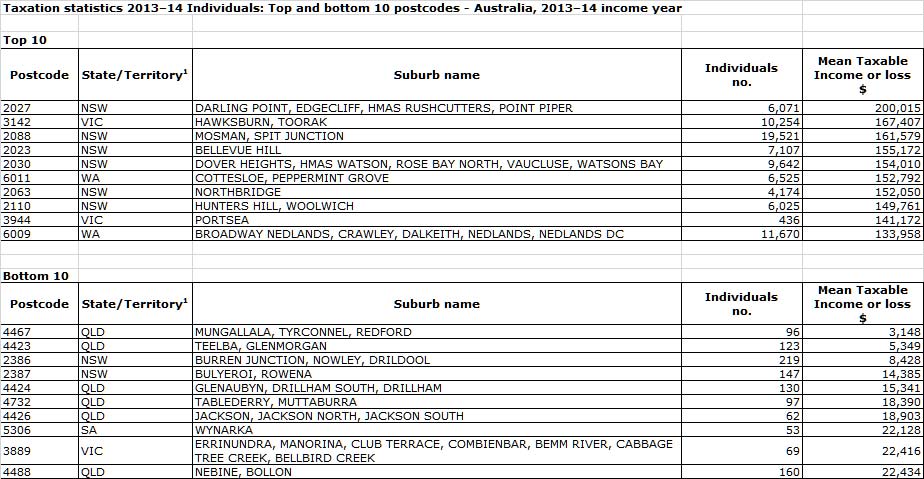
 Finally, here are the top and bottom 10 postcodes across the country.
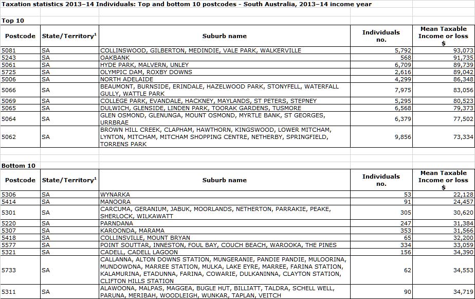
Adelaide Region Taxable Income Heat Map 2014
In our series of taxable income heat maps, using data from the ATO, from 2013-2014, today we look at Adelaide.
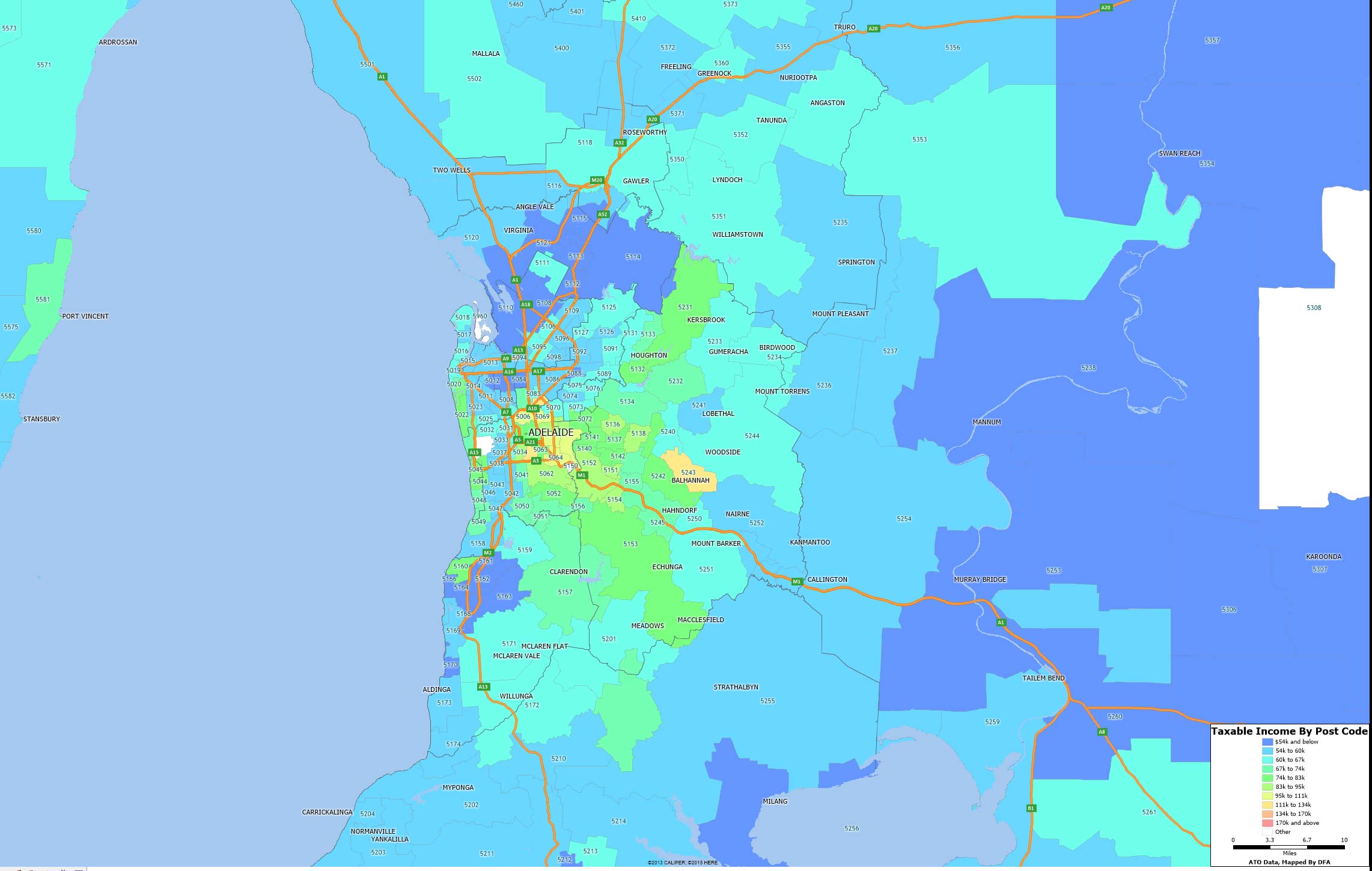 Here are the top and bottom 10 postcodes in the state.
More people moving to Victoria – ABS
Victoria is the most popular destination for people moving from other states. It is also Australia’s fastest growing state at 1.7 per cent, compared to an overall Australian growth rate of 1.3 per cent, according to figures released by the Australian Bureau of Statistics (ABS) today.
ABS Director of Demography, Beidar Cho said that over the year to September 2015, only Victoria and Queensland experienced net increases from interstate migration.
“Victoria gained 11,200 people from interstate migration which is up from 8,500 people in the previous year and Queensland gained 6,900 people, which is up from 5,900 people in the previous year,” Ms Cho said.
All the other states and territories recorded net interstate migration losses with New South Wales recording the largest loss with 7,500 people despite the state growing by 102,200 people over the year ending September 2015. Victoria narrowly exceeded NSW’s growth, with an increase of 102,300 people overall.
Prior to 2010, Victoria’s proportion of Net Overseas Migration (NOM) remained steady at approximately a quarter of all NOM to Australia. This began to change after 2012 when the proportion of NOM to Victoria and New South Wales began to climb as the proportion of NOM to Western Australia and Queensland began to drop. In the year ending September 2015 New South Wales continued to receive the highest proportion of NOM at 40 per cent. Victoria increased its proportion to 33 per cent of Australia’s total whilst WA and Queensland both received around 10 per cent.
Australia’s population grew by 313,200 people (1.3 per cent) to reach 23.9 million by the end of September 2015.
Net overseas migration contributed 167,700 people to the population (7 per cent lower than the previous year), and accounted for 54 per cent of Australia’s total population growth.
Net overseas migration was the major contributor to population change in New South Wales, Victoria and South Australia.
Over the year, natural increase contributed 145,600 people to Australia’s population, made up of 298,200 births (4 per cent lower than the previous year) and 152,700 deaths (1 per cent higher than the previous year).
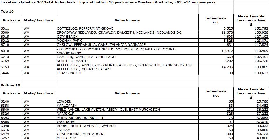
Perth Region Taxable Income Heat Map 2014
In our series of heat maps, using data from the ATO, today we look at Perth.
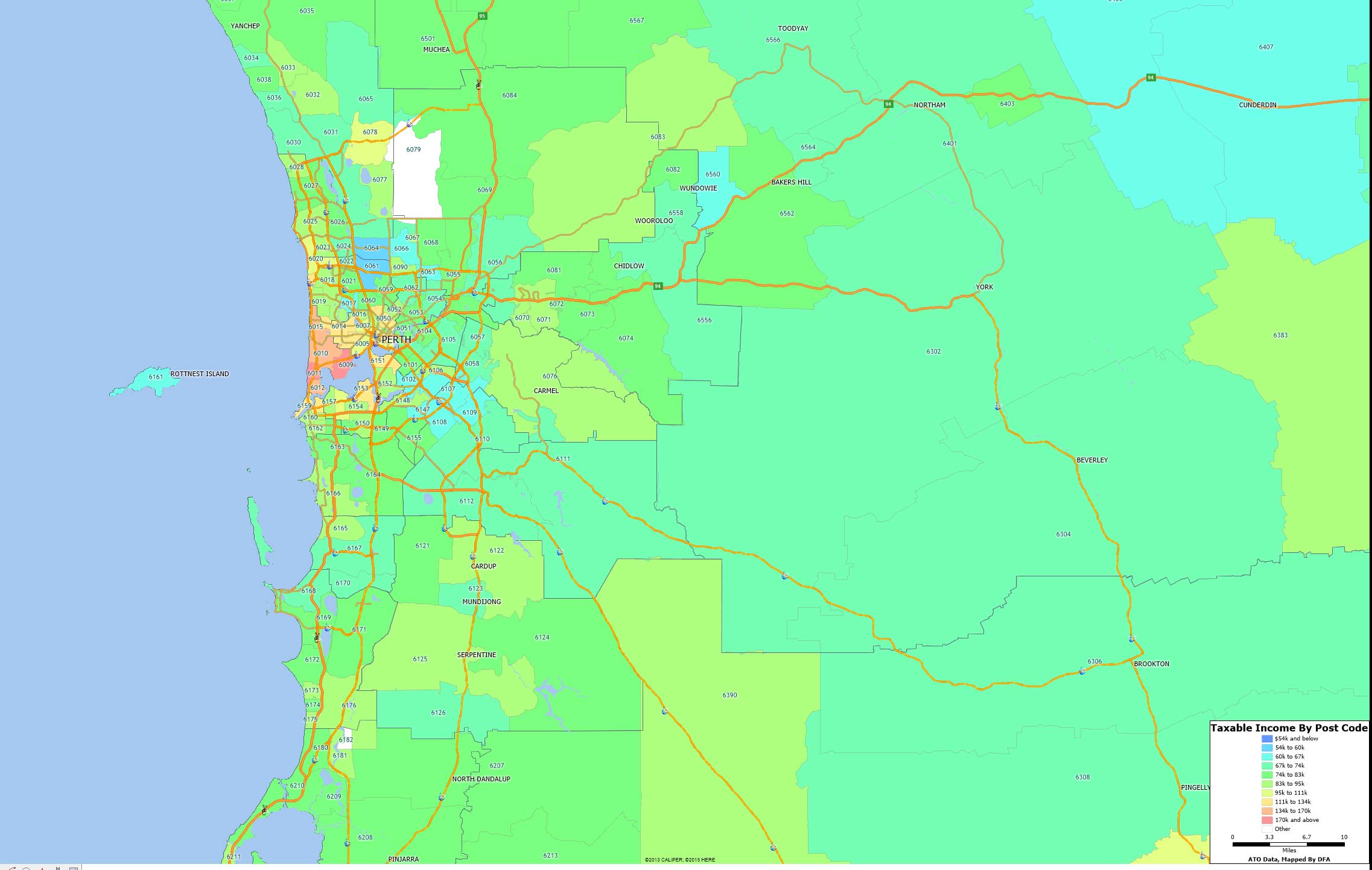 Here are the top and bottom post codes in WA.
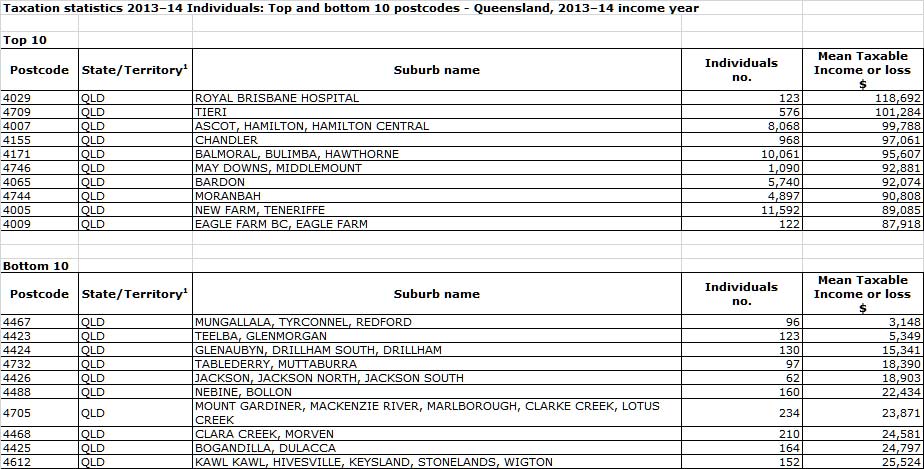
Brisbane Region Taxable Income Heat Map 2014
Continuing our feature on the recently released ATO data for 2013-2014, today we look at the taxable income heat map for the Brisbane region.
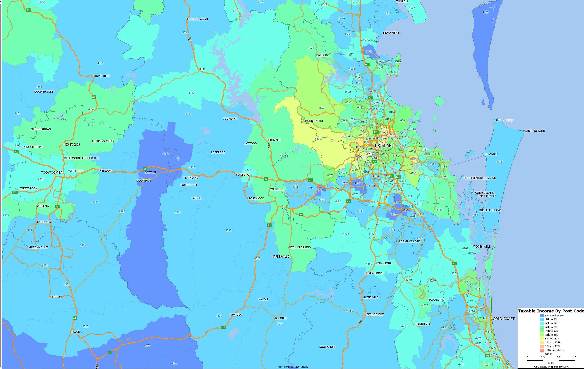 Here are to top and bottom post codes for the state.
Melbourne Region Taxable Income Heat Map 2014
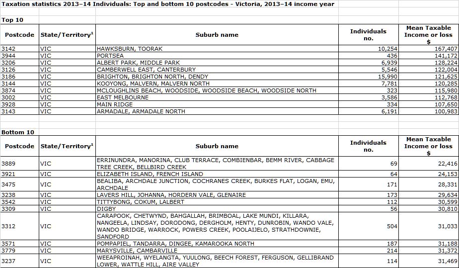
Continuing our heat mapping of the ATO taxable data by post code, today we feature Melbourne.
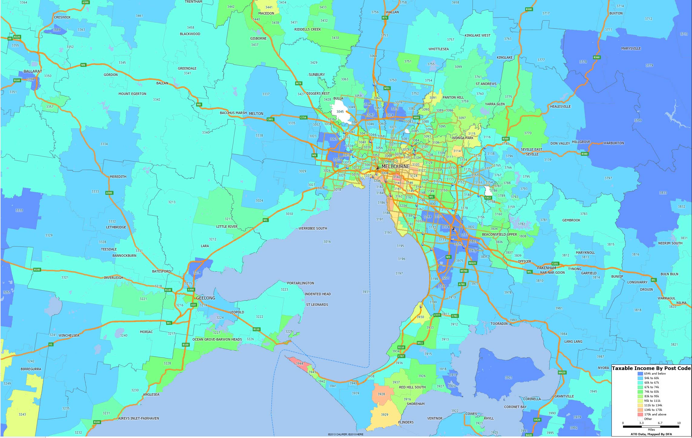 The top 10 and bottom 10 by post code are as follows: