How RBA Monetary Policy Works

In the June RBA Bulletin, there was an article which describes how the RBA executes its market interventions to effect a cash rate change. It is important to understand these inner workings, despite it appearing complicated on first blush.

And consider this, this tool box is being used by many central banks around the world to direct the financial system.

In summary, the RBA’s operations in domestic markets support the implementation of monetary policy. The most important tool to guide the cash rate to the target set by the Board is the interest rate corridor. To support this, the RBA pursues daily open market operations in order to keep the pool of exchange settlement (ES) balances at the appropriate level for the cash market to function smoothly. The daily market operations are conducted to offset the effects on liquidity of the many transactions between the banking system and the Australian Government. Open market operations are primarily conducted through repos and FX swaps. These provide flexibility for liquidity management and also help to manage risk for the RBA’s balance sheet.

The cash rate is a key determinant of interest rates in domestic financial markets and hence underpins the structure of the interest rates that influence economic activity and financial conditions more generally.

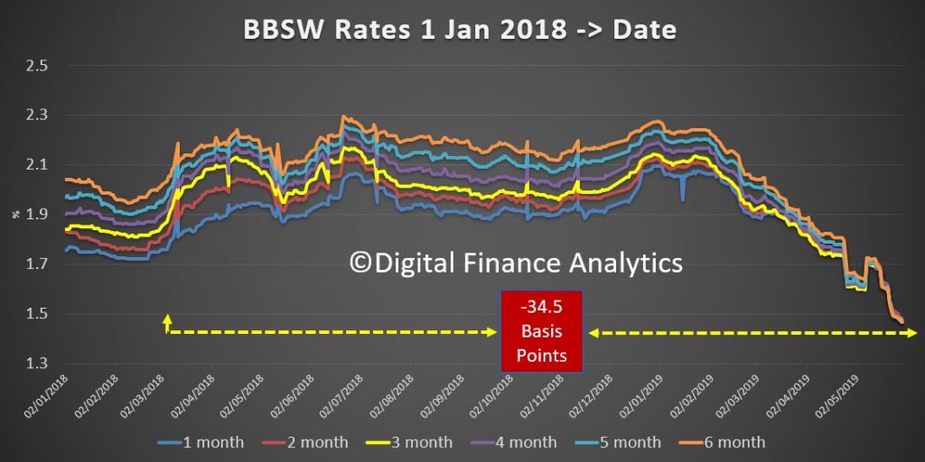
This helps to explain the sharp falls in the BBSW rates, which are now around 87 basis points lower than the recent peak. Such a fall has been engineered.

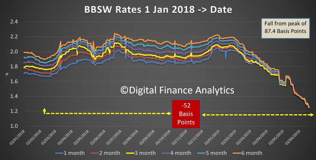
The cash rate is an effective instrument for implementing monetary policy because it affects the broader interest rate structure in the domestic financial system. The cash rate is an important determinant of short-term money market rates, such as the bank bill swap rate (BBSW), and retail deposit rates (Graph 1). These rates – as well as a number of other factors – then influence the funding costs of financial institutions and the lending rates faced by households and businesses. As a result, the cash rate influences economic activity and inflation, enabling the RBA to achieve its monetary policy objectives. However, while changes in the cash rate are very important, they are not the only determinant of market-based interest rates. Other factors, such as expectations, conditions in financial markets, changes in competition and risks associated with different types of loans are also important.

Graph 1: Interest Rates
Graph 1

The Cash Market and the Interest Rate Corridor

The RBA implements monetary policy by setting a target for the cash rate. This is the interest rate at which banks lend to each other on an overnight unsecured basis, using the exchange settlement (ES) balances they hold with the RBA. ES balances are at-call deposits with the RBA that banks use to settle their payment obligations with other banks. Banks are required to have a positive (or zero) ES balance at all times, including at the end of each day. It is difficult for institutions to predict whether they will have adequate funds at the end of any particular day, which generates the need for an interbank overnight cash market. Those banks that need additional ES balances after they have settled all payment obligations of their customers, borrow from banks with surplus ES balances. The interbank cash market is the mechanism through which these balances are redistributed between participants.

The RBA sets the supply of ES balances to ensure that the cash market functions smoothly by providing an appropriate level of ES balances to facilitate the settlement of interbank payments. The RBA manages the supply of ES balances available to the financial system through its open market operations (see below). Excessive ES balances could lead institutions to lend below the target cash rate, while a shortage might result in the cash rate being bid up above the target.

The interest rate corridor ensures that banks have no incentive to deviate significantly from the cash rate target when borrowing or lending in the cash market. Banks can borrow ES balances overnight on a secured basis from the RBA at a margin set 25 basis points above the cash rate target. As a result, banks have no need to borrow from other banks at a higher rate. Similarly, banks receive interest on their surplus ES balances at 25 basis points below the cash rate target. Therefore, they have no incentive to lend to other banks at a lower rate.

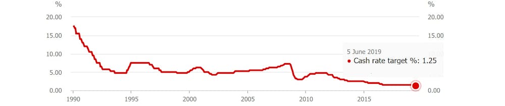
The operation of the interest rate corridor means that there is no need for the RBA to adjust the supply of ES balances to bring about a change in the cash rate (Graph 2 and Graph 3). For example, when the RBA lowered the cash rate target by 25 basis points from 1.5 per cent to 1.25 per cent in early June, the rates associated with the corridor also moved lower, to be 1.0 per cent on overnight deposits and 1.5 per cent on overnight loans (down from 1.25 per cent and 1.75 per cent). A bank that would have previously required a return above 1.25 per cent to lend ES balances in the cash market is, under the new corridor, willing to lend at a lower return. And so a bank wanting to borrow cash pays a lower rate than before. Similarly, if the RBA had instead raised the cash rate by 25 basis points from 1.5 per cent, the corridor would have moved up, to be 1.5 per cent to 2.0 per cent. A bank that would have previously lent surplus ES funds to another in the cash market at 1.50 per cent would, under the new corridor, no longer have an incentive to do so. Indeed, it would require a higher return to lend ES balances, rather than leaving those funds in its ES account and receiving 1.50 per cent from the RBA. Hence, a bank wanting to borrow in the cash market would have to pay a higher interest rate than it did previously.

In other words, interbank transactions automatically occur within the interest rate corridor without the RBA needing to undertake transactions beyond its usual market operations to manage liquidity.

Graph 2: Monetary Policy Easing
Graph 2
Graph 3: Monetary Policy Tightening
Graph 3

The incentives underlying the corridor guide the cash rate to the target and ordinarily all transactions occur at the rate announced by the RBA. The last time there was a small deviation in the published cash rate (which is a weighted average of all transactions in the cash market) from the target (of 1 basis point for two days) was in January 2010 (Graph 4). The lack of deviation of the cash rate from the target has brought about a self-reinforcing market convention where both borrowers and lenders in the cash market expect to transact at the prevailing target rate. This market convention helps to address the uncertainty that banks would otherwise face about the price at which they can borrow sufficient ES balances to cover their payment obligations each day. In 2018, daily transactions in the overnight interbank market were typically between $3 billion and $6 billion.

Graph 4: Cash Rate
Graph 4

As in Australia, many other central banks implement monetary policy with an interest rate corridor to guide the policy rate. The width of the corridor tends to differ, typically from 50 to 200 basis points. The choice of the width of the corridor is seen as a reflection of a trade‐off between interest rate control and the desire to avoid the central bank becoming an intermediary in the money market. All other things being equal, cross-country studies suggest that a narrower corridor is preferred by central banks that have a strong preference for low volatility of short-term interest rates, whereas a wider corridor is usually preferred by central banks that seek to encourage more interbank trading activity.

Over the past 10 years, many central banks (other than the RBA) have significantly expanded their balance sheets. This has resulted in significantly more liquidity in their respective systems and so banks typically do not need to borrow funds in the overnight cash market. In these cases, the policy rate typically converges toward the rate on deposits paid by the central bank; this is often referred to as a ‘floor system’. Small changes in liquidity in such a system do not tend to have much effect on the policy rate.

Liquidity Management and Open Market Operations

Transactions between the government (which banks with the RBA) and the commercial banks would, by themselves, change the supply of ES balances on a daily basis. ES balances in accounts of commercial banks increase whenever the government spends out of its accounts at the RBA. Similarly, when the government receives cash into its accounts at the RBA, such as from tax payments or debt issuance, ES balances decline. The RBA monitors and forecasts these changes actively through the day. It offsets (i.e. ‘sterilises’) these changes in ES balances with its daily open market operations so that government receipts and payments do not affect the aggregate level of ES balances. If transactions that affect system liquidity were not offset by the RBA, ES balances would be much more volatile and the payments system would suffer frequent disruptions (Graph 5). Ultimately this is likely to lead to a more volatile cash rate.

Graph 5: Surplus Exchange Settlement Balances
Graph 5

The main tools used in open market operations are repurchase (repo) agreements and foreign exchange swaps. Both repos and foreign exchange swaps involve a first and a second leg (Figures 1 and 2):

  • The first leg of a typical repo in open market operations (which injects ES balances) involves the RBA providing ES balances to a bank and the bank providing eligible debt securities as collateral to the RBA. Taking collateral safeguards the RBA against loss in the case of counterparty default. The second leg, which occurs at an agreed future date, unwinds the first leg: the bank returns the ES balances and the RBA returns the securities to the bank.
  • The first leg of a foreign exchange swap designed to inject ES balances into the system involves the RBA providing ES balances to a bank and the bank providing collateral in the form of foreign currency to the RBA (typically US dollars, euros or Japanese yen). The second leg, at the agreed future date, consists of the bank returning the ES balances and the RBA returning the foreign exchange.
Figure 1 Repurchase Agreement
Figure 1
Figure 2: Foreign Exchange Swap
Figure 2

Repos and swaps provide more flexibility for liquidity management than outright purchases or sales of assets since they involve a second leg (when the transaction unwinds) with a date chosen to support liquidity management on that day. It also allows the RBA to accept a much broader range of collateral, such as unsecured bank paper, than it would be willing to purchase outright. By contrast, buying (and then selling) securities outright requires the RBA to take on the price and liquidity risk associated with owning the assets outright. Conducting open market operations by buying and selling government securities outright, while also ensuring that the RBA’s market operations do not affect liquidity in the bond market, would require more government securities than are available in Australia.

The size of daily open market operations is based on forecasts of daily liquidity flows between the RBA’s clients (mainly the Australian Government) and the institutions with ES accounts. In a typical round of market operations, a public announcement is made at 9.20 am that the RBA is willing to auction ES balances against eligible collateral for a certain number of days (ranging from two days to several months, with an average term of around 30 days). Institutions have 15 minutes to submit their bid. The RBA ranks these bids from highest to lowest repo rate and then allocates ES balances to the highest bidders until the amount the RBA intends to auction has been dealt. All auction participants are informed electronically about their allocation. If they have been successful, they will pay the rate at which they bid for the amount allocated. The aggregate results of the auction, including the amount dealt, the average repo rate and the lowest repo rate accepted are published.

Market Operations and the RBA Balance Sheet

The transactions entered into as part of open market operations are reflected in changes in the RBA’s balance sheet. Changes in the size and composition of liabilities (mainly issuance of banknotes and government deposits) may need to be offset via open market operations to ensure that the availability of ES balances remains appropriate for the smooth functioning of the cash market (Graph 6).

Graph 6: Reserve Bank Liabilities
Graph 6

Open market operations affect the asset side of the balance sheet (Graph 7). When the RBA purchases securities under repo, it has a legal claim on the security that was transferred as collateral for the duration of the repo. These claims appear as assets on the balance sheet, along with outright holdings of domestic government securities. When the RBA uses foreign exchange swaps to supply Australian dollars into the local market, the foreign currency-denominated investments associated with the swap are also reflected as assets on the balance sheet. The choice between using repo, foreign exchange swaps or outright purchases to adjust the supply of ES balances is determined by market conditions and pricing. When a large amount of ES balances needs to be supplied or drained, such as when a government bond matures, the RBA might choose to do so using a combination of instruments.

Graph 7: Reserve Bank Assets
Graph 7

The RBA supplies ES balances not only for monetary policy implementation but also to facilitate the functioning of the payment system. Over recent years, the RBA has been providing more ES balances to banks to enable the settlement of payments outside normal banking hours, such as through direct-entry and the New Payments Platform. These ES balances are supplied under ‘open repos’. An open repo is set up in a similar way to the repo explained in Figure 1, with the initial leg transferring ES balances to banks in return for eligible debt securities as collateral. However, the date of the second leg is not specified, so it is open ended. The ES balances are available (and the claim on securities remain on the RBA’s balance sheet) until the open repo is closed out. These ES balances provided under open repo are held purely to facilitate the effective operation of the payments system after hours and cannot be lent overnight in the cash market. As a result, they have no implications for the implementation of monetary policy. Currently, these balances are around $27 billion. The remainder of ES balances that are available for trading in the cash market are referred to as ‘surplus ES balances’, and are the focus of daily open market operations. Recently, surplus ES balances have been around $2–3 billion. This amount has increased in recent years as demand for balances has risen, partly in response to new prudential regulations on liquidity.

RBA Penny Drops On Underemployment (Just A Decade Late)

RBA Governor Philip Lowe spoke at CEDA today. He signals more rate cuts, their potential limited impact and the need for other strategies to move towards higher levels of employment. Underemployment makes an entrance – finally! We have been talking about this for years.

Today, I would like to explain why this is so and also discuss how we assess the amount of spare capacity in the labour market. I will then finish with some comments on monetary policy.

The Broad Policy Framework

Students of central bank history would be aware that the Reserve Bank Act was passed by the Australian Parliament in 1959 – 60 years ago. In terms of monetary policy, the Parliament set three broad objectives for the Reserve Bank Board. It required the Board to set monetary policy so as to best contribute to:

  1. The stability of the currency
  2. The maintenance of full employment
  3. The economic prosperity and welfare of the people of Australia

These objectives have remained unchanged since 1959. Here, in Australia, we did not follow the fashion in some other parts of the world over recent decades of setting just a single goal for the central bank – that is, inflation control. In my view it was very sensible not to follow this fashion. Our legislated objectives – having three elements – are broader than those of many other central banks. The third of our three objectives serves as a constant reminder that the ultimate objective of our policies is the collective welfare of the Australian people.

From an operational perspective, though, the flexible inflation target is the centre piece of our monetary policy framework. The target – which has been agreed to with successive governments – is to deliver an average rate of inflation over time of 2–3 per cent. Our focus is on the average and on the medium term.

Inflation averaging 2 point something constitutes a reasonable definition of price stability. Achieving this stability helps us with our other objectives. Low and stable inflation is a precondition to the attainment of full employment and it promotes our collective welfare. As I have said on other occasions, we are not targeting inflation because we are inflation nutters. Rather, we are doing so because delivering low and stable inflation is the most effective way for Australia’s central bank to promote our collective welfare.

So where does the labour market fit into all this?

The answer is that it is central to all three objectives.

The connection with the second objective – full employment – is obvious. The RBA is seeking to achieve the lowest rate of unemployment that can be sustained without inflation becoming an issue. In doing this, one of the questions we face is what constitutes full employment in a modern economy where work arrangements are much more flexible than they were in the past. I will return to this issue in a moment.

The labour market is, of course, also central to the third objective in our mandate – our collective welfare. It is stating the obvious to say that for many Australians, having a good job at a decent rate of pay is central to their economic prosperity.

Trends in the labour market also have a major bearing on inflation outcomes, so they are important for the first element of our mandate as well. Over time, there is a close link between wages growth and inflation. And a critical influence on wage outcomes is the balance between supply and demand in the labour market; or in other words how much spare capacity is there in the labour market? This question is closely linked to the one about what constitutes full employment.

So, it is natural that we focus on the labour market as the Board makes its monthly decisions about interest rates.

Spare Capacity

With that background I would now like to discuss how we assess the degree of spare capacity in the Australian labour market. I will do this from four perspectives:

  1. The rates of unemployment and underemployment
  2. The flexibility of labour supply
  3. The effectiveness with which people are matched with job vacancies
  4. Trends in wages growth.

Unemployment and underemployment

The conventional measure of spare capacity in the labour market is the gap between the actual unemployment rate and the unemployment rate associated with full employment. Even at full employment, some level of unemployment is to be expected as workers leave jobs and search for new ones. As my colleague Luci Ellis discussed last week, we don’t directly observe the unemployment rate associated with full employment – we need to estimate it.[1] Over recent times there has been a gradual accumulation of evidence which has led to lower estimates. While it is not possible to pin the number down exactly, the evidence is consistent with an estimate below 5 per cent, perhaps around 4½ per cent. Given that the current unemployment rate is 5.2 per cent, this suggests that there is still spare capacity in our labour market.

The fact that the conventional estimate of spare capacity is based on the unemployment rate reflects an implicit assumption that if you have a job you are pretty much fully employed. In decades past, this might have been a reasonable assumption. But it is not a realistic assumption in today’s modern flexible labour market.

As more people work part time, it has become increasingly common to be both employed and to work fewer hours than you want to work. In the 1960s, less than one in ten workers worked part time (Graph 1). Today, one in three of us works part time. Almost one in two women work part time and more than one in two younger workers work part time.

Graph 1: Part-time Workers
Graph 1

A few more facts are perhaps helpful here. According to the ABS, around 3 million people work part time because they want to, not because they can’t find a full-time job. Most people who are working part time do so because they are studying or have caring responsibilities, or for other personal reasons. So we should not think of part-time jobs as being bad jobs, and full-time jobs as being good jobs. Rather, one of the success stories of the Australian labour market is that we have been able to accommodate this desire for part-time work and flexibility.

Having said that, around one-quarter of people working part time are not satisfied with the hours they are offered and would like to work more hours: we can think of these people as underemployed (Graph 2). The share of part-time workers who are underemployed moves up and down from year to year, and the current share is above its average level over the past two decades.

Graph 2: Part-time Underemployment
Graph 2

As part of the ABS’s monthly survey of 50,000 people, it asks underemployed workers how many extra hours they would like to work. On average, they answer that they would like to work an extra 14 hours per week. It is interesting that this figure has trended down over the past two decades; it used to be more than 16 hours. Over the same period, the average hours worked by part-time workers has increased by around 2 hours to 17 hours per week. Taken together, these data suggest that businesses are doing a better job of providing the hours that part-time workers are seeking.

This shift to part-time work means that in assessing spare capacity we need to consider measures of underemployment as well as measures of unemployment. The RBA has been doing this for some time. As part of our efforts here, we have constructed a measure of underutilisation that takes account of the part-time workers who want to work more hours. This measure adds the extra hours sought by these workers to the hours sought by those who are unemployed (Graph 3).[2] These extra hours are equivalent to around 3.3 per cent of the labour force, which, taking account of conventional unemployment, means that the underutilisation rate is 8.1 per cent. This hours-based measure is preferable to heads-based measures of underutilisation that treats an unemployed person in the same way as a part-time worker seeking a few more hours.

Graph 3: Hours-based Labour Underutilisation
Graph 3

Unlike the unemployment rate, which has trended down over the past 20 years, the underemployment rate has been relatively stable. These different patterns in unemployment and underemployment suggest that fewer inroads have been made into spare capacity in the labour market than suggested by looking at the unemployment rate alone. This is something we take into account in thinking about monetary policy.

There is, though, one other perspective on the measure of underemployment that I would like to share with you. In the past, when part-time work was not as readily available, many people – mostly women – faced the choice of taking full-time paid employment or no paid employment at all. Many chose to, or had to stay outside the labour force because working was not a realistic option. From the perspective of society as a whole, this was a serious form of underutilisation – it just wasn’t measured as such by the ABS.

Given the trend towards part-time and more flexible jobs, people have more options than they had before and many have chosen to join, or have deferred leaving, the labour force.[3] From the perspective of adding to the productive capacity of the nation, this is a good outcome and if there was a measure of underutilisation that took account of exclusion from the workforce, it would surely have declined. I don’t want to downplay the issue of underemployment, but it is worth recognising this broader perspective, and remembering where we have come from.

Flexibility of the supply side

This naturally brings me to my second window into spare capacity in the labour market – the flexibility of labour supply.

Over the past 2½ years, the working-age population has increased at an annual rate of around 1¾ per cent. Over that same time period, employment has increased at an average rate of 2¾ per cent. The fact that employment has been increasing considerably faster than the working-age population has led to a reduction in the unemployment rate, but the reduction is not as large as might have been expected. The reason for this is that the supply of labour has increased in response to the stronger demand for workers.

This flexibility in labour supply is evident in the substantial rise in labour force participation. The participation rate currently stands at 66 per cent, which is the highest on record (Graph 4). Reflecting this, the share of the working-age population in Australia with a job is currently around the record high it reached at the peak of the resources boom. As I discussed a few moments ago, the availability of part-time and flexible working arrangements is one reason for this.

Graph 4: Participation and Employment Ratios
Graph 4

There are two groups for which the rise in participation has been particularly pronounced: women and older Australians (Graph 5). The female participation rate now stands at 61 per cent, up from 43 per cent in 1979. Australia’s female participation rate is now above the OECD average, although it remains below that of a number of countries, including Canada and the Netherlands.

The participation rate of older workers has also increased over recent decades as health outcomes have improved and changes have been made to retirement policies. The eligibility age for the pension was progressively raised from 60 to 65 for females and is now being gradually increased to 67 for everybody by 2023. The preservation age at which individuals can access their superannuation is also being gradually increased. These changes are contributing to higher participation by older Australians.

Graph 5: Participation Rate
Graph 5

Another source of potential labour supply is net overseas migration. Migration, including temporary skilled workers, increased sharply during the resources boom when demand for skilled labour was very strong, and has subsequently declined (Graph 6). While migrants add to both demand and supply in the economy, they can be a particularly important source of capacity for resolving pinch-points where skill shortages exist.

Graph 6: Temporary Resident (Skilled) Visas Granted
Graph 6

A related source of flexibility stems from our unique relationship with New Zealand. When labour demand is relatively strong in Australia, there tends to be an increase in the net inflow of workers from New Zealand to Australia. When conditions are relatively subdued here, the reverse occurs. During the resources boom, the inflow from across the Tasman were as large as the inflow of temporary skilled workers.

The overall picture here is one of a flexible supply side of the labour market. When the demand for labour is strong, more people enter the jobs market or delay leaving. This rise in participation is a positive development. But it is one of the factors that has meant that strong demand for labour has not put much upward pressure on wages.

The matching of people with jobs

A third perspective on spare capacity in the labour market can be gained from examining how well people looking for jobs are matched with the jobs that are available. Looking at the labour market from this perspective, things look a little tighter than suggested by the other two perspectives that I have discussed.

Currently, almost 60 per cent of firms report that the availability of labour is either a minor or a major constraint on their business (Graph 7). This share is not as high as it was during the resources boom, but it is still quite high. Reports from the RBA’s liaison program suggest that there are currently shortages of certain types of engineers, workers with specialised IT skills and some tradespeople associated with public infrastructure work. Businesses in regional areas are also more likely to report a greater degree of difficulty finding suitable labour.

Graph 7: Difficulty Finding Suitable Labour
Graph 7

One contributing factor here is an underinvestment in staff training. In the shadow of the global financial crisis many firms cut back training to reduce costs. We are now seeing some evidence of the adverse longer-term implications of this. As the labour market tightens further, I would hope that more firms are prepared to hire workers and provide the necessary training.

Another lens on job matching is the ratio of the number of unemployed people to the number of job vacancies (Graph 8). At present, there are fewer than three unemployed people for each vacancy. This compares with over 20 people for every vacancy in the early 1990s recession and five people for every vacancy in 2014. From this perspective the labour market looks reasonably tight. There is also some tentative evidence that, on average, unemployed workers are not as well matched to job vacancies as was the case in 2007, when the ratio of the two was at a similar level.

Graph 8: Unemployment-to-vacancies-Ratio
Graph 8

One such piece of evidence is that as the unemployment rate has come down over recent years, there has been little progress on reducing very long-term unemployment, defined as those who are unemployed for more than two years (Graph 9). Addressing the causes of this chronic unemployment remains an important challenge for our community. More positively, the share of the labour force that has been unemployed between one and two years has trended down over recent times.

Graph 9: Long-term Underemployment Rates
Graph 9

Another lens on job matching and the overall tightness of the labour market is the rate of job mobility; that is, how often people change their jobs. Here, the evidence is interesting. Despite the frequent reports of a lack of job security and regular job switching by millennials, the average time that workers are staying with an employer is increasing. Reflecting this, the share of employed people who switch employers in a given year is the lowest it has been in a long time (Graph 10). Looking at the data by occupation, the rate of job mobility is lowest for managers and business professionals and highest for tradespeople and workers in the hospitality industry.

Graph 10: Job Mobility
Graph 10

In a tight labour market, we would expect to see either strong wages growth or frequent job changing as businesses seek out workers. But we are seeing neither at present. One possible explanation for this is the uncertainty that many people feel about the future. This uncertainty means that if you have a job you want to keep it rather than take a risk with a new employer. This might be especially so if you also have a large mortgage. So it is possible that the high level of household debt is also affecting labour market dynamics.

Wages

I will now turn to the fourth perspective on labour market tightness – that is wages growth.

Over the past year, wages growth has picked up as the labour market tightened. This is not surprising given the strength of demand for labour. But the pick-up has been fairly modest and is only evident in the private sector (Graph 11). Over the past year, the private-sector Wage Price Index increased by 2.4 per cent, up from 1.9 per cent in the previous year. The past two quarters have, however, seen lower wage increases than in the previous two quarters.

In contrast to trends in the private sector, wages growth in the public sector has been steady at around 2½ per cent, largely reflecting the wage caps across much of the public sector.

It is also worth pointing out that overall wages growth in New South Wales and Victoria has been running at just 2½ per cent despite the unemployment rate being 4½ per cent or lower over the past year.

Graph 11: Wage Price Index Growth by Sector
Graph 11

Another perspective on wages growth is from the national accounts, which reports average earnings per hour worked (Graph 12). This measure is volatile, but the latest data painted a fairly weak picture, with average hourly earnings up by just 1 per cent over the past year.

Graph 12: Labour Costs
Graph 12

In summary, the overall picture from these various windows into the labour market is that despite the strong employment growth over recent times, there is still considerable spare capacity in the labour market. We remain short of the unemployment rate associated with full employment, there is significant underemployment and there is further potential for labour force participation to increase when the jobs are there. Consistent with all of this, wages growth remains modest and is below the rate that would ensure that inflation is comfortably within the 2 to 3 per cent range. The one caveat to this assessment is the difficulty that some firms are having finding workers with the necessary skills. This underlines the importance of workplace training.

Monetary Policy

I would like to finish with a few words on monetary policy.

As you are aware, the Reserve Bank Board reduced the cash rate to 1¼ per cent at its meeting earlier this month. This was the first adjustment in nearly three years.

This decision was not in response to a deterioration in the economic outlook since the previous update was published in early May. Rather, it reflected a judgement that we could do better than the path we looked to be on.

The analysis that I have shared with you today supports the conclusion that the Australian economy can sustain a higher rate of employment growth and a lower unemployment rate than previously thought likely. Most indicators suggest that there is still a fair degree of spare capacity in the economy. It is both possible and desirable to reduce that spare capacity. Doing so will see more people in jobs, reduce underemployment and boost household incomes. It will also provide greater confidence that inflation will increase to be comfortably within the medium-term target range.

Monetary policy is one way of helping get us onto to a better path. The decision earlier this month will assist here. It will support the economy through its effect on the exchange rate, lowering the cost of finance and boosting disposable incomes. In turn, this will support employment growth and inflation consistent with the target.

It would, however, be unrealistic to expect that lowering interest rates by ¼ of a percentage point will materially shift the path we look to be on. The most recent data – including the GDP and labour market data – do not suggest we are making any inroads into the economy’s spare capacity. Given this, the possibility of lower interest rates remains on the table. It is not unrealistic to expect a further reduction in the cash rate as the Board seeks to wind back spare capacity in the economy and deliver inflation outcomes in line with the medium-term target.

It is important though to recognise that monetary policy is not the only option, and there are limitations to what can be achieved. As a country we should also be looking at other ways to get closer to full employment. One option is fiscal policy, including through spending on infrastructure. Another is structural policies that support firms expanding, investing, innovating and employing people. Both of these options need to be kept in mind as the various arms of public policy seek to maximise the economic prosperity of the people of Australia.


RBA Untroubled By Mortgage Arrears {Gasp}

The RBA’s Jonathan Kearns, Head of Financial Stability Department spoke to the Property Council. He said that the share of banks’ housing loans in arrears is now back around the level reached in 2010, the highest it has been for many years. But arrears are still well below the level reached in the early 1990s recession. But… we are NOT in recession….??? He concludes that housing arrears have risen but by no means to a level that poses a risk to financial stability. But as he says, mortgage arrears can be associated with significant personal trauma for borrowers.

I want to address an important issue for the property industry – the rising rate of housing loan arrears (Graph 1). Why is it that an increasing share of housing borrowers are behind in their mortgage repayments? Mortgage arrears can be associated with significant personal trauma for borrowers. They also point to a rising risk to the financial system as housing loans are 40 per cent of banks’ assets. If the value of the property backing the loan exceeds the value of the loan then arrears won’t have a big impact on banks’ profits or capital. But with falling housing prices the potential for banks to experience losses increases. So, on several fronts, this is an important issue.

Graph 1: Banks' Non-performing Household Loans
Graph 1

There are many reasons why borrowers fall into arrears, almost all of which involve a fall in income or rise in expenses – or both. Some borrowers experience personal misfortune, such as ill health or a relationship breakdown, which is unrelated to economic conditions or the quality of their loan. And even in good times, some people become unemployed. So there will always be some borrowers who fall into arrears.

However, it is weak economic conditions that drive cyclical upswings in arrears. In particular, borrowers can struggle to make their payments if their income falls. Weak conditions in housing markets make it hard for borrowers to get out of arrears by selling their property. Conversely, large increases in interest rates, say to slow an overheating economy, can also contribute to rising arrears.

Banks’ lending standards also play a role in arrears. And it is important to note that economic conditions and lending standards interact. Poorer quality loans might continue to perform well in good economic conditions, and only fall into arrears with an economic downturn. In contrast, good quality loans will be more resilient in a downturn.

Because of the interaction between the various drivers of arrears, we often cannot point to a single cause of rising arrears. Today I want to discuss the ways in which economic conditions and lending standards are pushing arrears rates higher.

How High Are Arrears?

But first, it’s worth pausing to compare some benchmarks for the level of arrears. The share of banks’ housing loans in arrears is now back around the level reached in 2010, the highest it has been for many years. But arrears are still well below the level reached in the early 1990s recession.[1]

While the increase in arrears and its level is notable, the rate of arrears in Australia is still relatively low internationally, and in an absolute sense. The available data indicate that arrears are lower in Australia than in many other advanced economies (Graph 2). Indeed, another way to look at the arrears rate in Australia is to note that over 99 per cent of housing loans are on, or ahead of, schedule. Making loans involves risk, and banks are used to managing this risk. If the arrears rate was persistently very low, that would suggest that lenders were being too cautious in lending. In that world, some people who could almost certainly repay a loan would struggle to get one.

Graph 2: Non-performing Household Loans
Graph 2

Borrower Income

So what drives arrears? Income is a major determinant of whether borrowers can meet their repayments. Strong employment growth for a number of years now has seen the unemployment rate decline. On the surface, this makes it surprising that rates of arrears have been rising. But the relationship between unemployment, income and arrears isn’t straightforward.

One factor at play is that, while the unemployment rate has declined nationally, this hasn’t been the case everywhere. What we can see across Australia is there is a clear pattern of more loans going into arrears in locations where the unemployment rate is higher (Graph 3). Notably the unemployment rate has increased and income growth slowed in Western Australia and parts of Queensland with the end of the mining boom. These areas have seen larger increases in arrears. In Western Australia the arrears rate is now around double the rate in the rest of the country. But the flow of loans into arrears in these regions is more than would be suggested by the unemployment rate alone.

Graph 3: Unemployment and Arrears
Graph 3

Indeed, rising unemployment in some areas can’t be the whole story. As I said, the national unemployment rate has declined in recent years. So, when it comes to arrears, falling unemployment in some regions has not compensated for rising unemployment in others. One explanation is that it can matter who becomes unemployed and who gains a job. People aged in their thirties and forties are more likely to have a mortgage, particularly if they have good employment prospects. So, if more of them become unemployed, arrears rates will rise. Conversely, if it is older or younger workers who get a job, but don’t have a mortgage, or second income earners in households already comfortably making their repayments, this won’t lead to a decline in arrears rates.

The length of unemployment can also influence arrears. Around two-thirds of borrowers have accumulated buffers of prepayments of their mortgage, and some others have other assets outside of their property. Households with financial buffers can withstand some period of unemployment, but if that extends too long and depletes their savings, they risk falling into arrears.

There are several other reasons why focusing on unemployment doesn’t tell the full story. It isn’t that all borrowers either receive income or don’t. Often borrowers may lose some of their income, say because of reduced work hours, a smaller bonus or because tenants move out of their investment property. When they don’t have a large income or savings buffer, even small income falls or an unexpected increase in expenditure can put borrowers into arrears. Indeed in Western Australia where arrears have increased most, rental property vacancy rates have been high, reducing the income of landlords.

The rate of growth of income can play a role too. When nominal income is rising strongly, over time, mortgage payments take up a declining share of a borrower’s income. As their mortgage ages and their income rises, borrowers are better placed to withstand a fall in their income or rise in expenses. Over the past five years, nominal income growth has been around half its longer-run average.[2] So, rising income hasn’t been able to compensate for other factors that might cause households to struggle to make their mortgage repayments.

Housing Prices

Another recent feature of arrears is that, on average, mortgages are staying in arrears for longer. There are several possible explanations for this. Mortgages can leave arrears because the lender takes possession of the property and sells it. However, the number of repossessed mortgaged properties is very small and if anything has risen slightly, so this can’t explain longer loan arrears.

Alternatively, borrowers can leave arrears by selling their property and repaying the loan.[3] In a strong housing market it is easy for borrowers struggling to make repayments, or already in arrears, to sell their property. In a strong housing market, it doesn’t take long to sell a property at an attractive price. The owner is also likely to have had several years of price growth, increasing their equity. So if they sell they are better placed to pay off their mortgage and still have some of their savings.

But nationally prices have fallen 8 per cent from their peak, auction clearance rates and volumes have declined, and properties are taking longer to sell. In this environment, borrowers who fall into arrears find it harder to sell their property and repay their loan (Graph 4). Indeed, across the country, we see there is a strong relationship between recent housing price growth and the rate at which borrowers are leaving arrears. In those locations where housing price growth has been weaker, a smaller share of borrowers transition out of arrears.

Graph 4: Exits from Arrears and Housing Price Growth
Graph 4

Other Economic Factors

The weaker housing market has also seen housing credit growth slow. Because loans tend to take some time to go into arrears, this has the effect of reducing the number of new loans that have repayments on schedule, and so increases the overall arrears rate. But our estimates suggest that slower credit growth accounts for less than one-tenth of the increase in the arrears rate since early 2016.

Another driver of arrears can be changes in interest rates. In the period before the GFC, arrears rates were rising despite strong economic conditions, in part because of large increases in mortgage interest rates. However, in recent years, interest rates on outstanding mortgages have been declining and so average mortgage interest rates have not contributed to the generalised increase in arrears.

Lending Standards

Lending standards are also an important driver of arrears rates. Weaker lending standards mean that borrowers can get larger loans and more borrowers get loans with potentially riskier characteristics, such as interest only periods. For a borrower, the larger their required loan repayments relative to their available income, the slower they will be able to build up a buffer, and so the more likely they are to fall into arrears if their income falls or expenses rise. With weaker lending standards, more loans will be made to borrowers who are likely to experience difficulty repaying their loan, say because their income is less stable. For these reasons, weaker lending standards can lead to higher rates of arrears.

In Australia there has been a significant tightening of housing lending standards by the regulators of banks and other lenders, in earnest from around 2014. Regulators took these actions amid concerns that strong housing market conditions and strong competition by lenders had seen lending standards erode. The actions taken by the Australian Prudential Regulation Authority (APRA) included that banks apply more stringent interest rate buffers to maximum loan size calculations, increase their scrutiny of borrowers’ income and expenses, and reduce their share of lending with high loan-to-valuation ratios (LVRs). Complementing this, the Australian Securities and Investments Commission (ASIC) increased their focus on lenders’ compliance with responsible lending obligations, particularly in the area of interest-only lending.[4] These actions were designed to ensure that lenders only extend as much debt to borrowers as they will be able to repay, including a buffer.

Tighter lending standards should lead to lower arrears but this can take time to show up. Typically borrowers’ financial pressures build over time and so average arrears rates increase with time since loan origination, that is with ‘loan seasoning’.[5] For example, a three-year old loan is four times more likely to go into arrears than a one-year old loan. Another challenge of assessing the impact of lending standards on arrears is that different cohorts of loans experience common macroeconomic conditions at different times in their seasoning. If there is a sharp increase in unemployment in a given year, the cohort of loans originated one year earlier experience this with only 12 months of seasoning, while the cohort originated three years earlier experience it with 36 months of seasoning. This suggests that more recent loans would likely have a larger increase in arrears in response to rising unemployment.

Using the Reserve Bank’s Securitisation Dataset we find evidence consistent with more recent cohorts of loans having lower arrears rates than earlier cohorts. Specifically, those loans originated in the past few years have an arrears rate that is up to one-quarter of a percentage point lower than loans originated prior to 2014 (controlling for seasoning and common time effects such as the state of the economy) (Graph 5).[6] The lower arrears rates for more recent loans suggests these tighter lending standards have been effective.

Graph 5: Arrears Rates by Origination Year
Graph 5

However, in other ways, measures taken to improve lending standards may actually temporarily increase arrears rates. One measure addressed the large and increasing share of loans that were interest only, meaning the borrower was not required to make regular principal payments and so the loan size did not necessarily decline over time. In 2017, APRA imposed a 30 per cent benchmark for the maximum share of lenders’ new loans that could be interest only. That benchmark has since been removed. But, recognising the greater risk of interest-only lending, banks continue to charge higher interest rates for these loans and more carefully scrutinise their suitability for borrowers. As a result, some borrowers who may have anticipated being able to roll over an interest-only period are finding they cannot. Some are then facing temporary difficulty servicing the higher principal and interest (P&I) payments at the end of the interest-only period. However, most borrowers in this position get their repayments back on track within a year.

Tighter lending standards have made it more difficult for some borrowers to refinance their loan. In general, a borrower who, say, experienced a decline in their income may be able to reduce their repayments by refinancing with a loan that is at a lower interest rate or has a longer term and so lower repayments. But borrowers who are financially stretched are more likely to be constrained by tighter borrowing restrictions. If they can’t refinance and struggle to make their existing repayments, they are more likely to fall into arrears.

There have also been some reports that banks have been displaying greater forbearance, that is, allowing loans to stay in arrears for longer. Supposedly, this is in response to a recognition of, and attention on, some past poor lending decisions. However, it seems unlikely that this could explain a significant part of the increase in aggregate arrears. In an environment of falling housing prices, allowing a borrower to remain in arrears for longer would increase the loss that the borrower, and so the lender, is exposed to. This wouldn’t seem to be operating in the best interests of the borrower, or for that matter even the lender.

Conclusion

Summing up, housing arrears have risen but by no means to a level that poses a risk to financial stability. Several factors have been interacting to drive the rise in housing arrears. Economic conditions are undoubtedly part of the story. Weak income growth, housing price falls and rising unemployment in some areas have all contributed. But they have not acted alone, interacting with earlier weaker lending standards, and the more recent tightening in lending standards. To the extent that we can point to drivers of the rise in arrears, while the economic outlook remains reasonable and household income growth is expected to pick up, the influence of at least some other drivers may not reverse course sharply in the near future, and so the arrears rate could continue to edge higher for a bit longer. But with overall strong lending standards, so long as unemployment remains low, arrears rates should not rise to levels that pose a risk to the financial system or cause great harm to the household sector.

RBA Minutes – 4.5% Unemployment Target Means More Rate Cuts Ahead [Never Mind Savers!]

The RBA released their minutes today which clearly signals further rate cuts ahead as they drive toward to goal of 4.5% unemployment – the latest magic figure when wages will start to rise. Savers be dammed, to try and get household spending up.

International Economic Conditions

Members commenced their discussion by noting that the data on the global economy released since the previous meeting had been mixed. GDP growth outcomes for the March quarter in some economies had been slightly stronger than the second half of 2018, while labour markets had remained tight. However, global trade and conditions in the global manufacturing sector had remained weak. New export orders had been little changed at subdued levels and growth in industrial production had slowed in many economies, including those economies in east Asia that are closely integrated with global supply chains.

The US–China trade dispute had escalated in May, intensifying the downside risk posed to the global economic outlook from this source. The United States had proceeded to increase tariffs from 10 per cent to 25 per cent on US$200 billion of imports from China, and China had responded by announcing that tariffs would increase by 5–25 per cent on US$60 billion of US imports from 1 June 2019. In the days leading up to the meeting, the US administration had also announced tariff measures affecting Mexico and India.

In the major advanced economies, GDP growth for the March quarter had been somewhat stronger than in the second half of 2018. However, in both Japan and the United States the contribution from domestic demand had declined, and investment intentions in Japan pointed to only moderate investment growth over the period to early 2020. Nevertheless, labour markets in the advanced economies had remained tight. As a result, wages growth had continued to increase, reaching around the highest rates recorded during the current expansion in the three major advanced economies. Moreover, firms’ employment intentions had remained positive at high levels and firms had continued to report widespread difficulties in filling jobs.

Inflation had remained subdued globally despite tight labour markets and rising wages growth in many advanced economies. Core inflation had been below target in the three major advanced economies, following the decline in core inflation in the United States in recent months. Members noted that temporary factors had been contributing to the decline in the US core inflation measure, with the trimmed mean underlying inflation measure close to 2 per cent over recent months.

In China, indicators of activity had moderated in April. The moderation had partly reversed the unusually strong results in March, which had included activity brought forward ahead of tax changes that came into effect on 1 April 2019. Growth in fixed asset investment had slowed in April, driven by a sharp fall in manufacturing investment, while infrastructure investment had been supported by increased government spending. Industrial production had slowed across a wide range of products in April, although production of construction-related materials – such as steel, plate glass and cement – had remained strong.

Elsewhere in east Asia, growth had slowed further in the March quarter, mainly because of weaker growth in exports and investment. Growth in India had been at the lower end of the range of recent experience, with members noting that the recent tariff announcements by the US administration could adversely affect Indian exports of goods.

Commodity price movements had been mixed since the previous meeting. Iron ore and rural prices had increased. The increase in iron ore prices had been underpinned by supply constraints, strong demand from China and an increase in steel production. On the other hand, the prices of coal, oil and base metals had declined. Members noted that the decline in oil prices had mainly reflected renewed concerns around the outlook for global oil demand.

Domestic Economic Conditions

Members noted that national accounts data for GDP growth in the March quarter would be released the day after the meeting. GDP growth was expected to have been a little firmer than in the preceding two quarters, supported by growth in exports, non-mining business investment and public spending. Growth in consumption, however, was expected to continue to be sluggish and dwelling investment was expected to have declined further in the March quarter.

Information received for the June quarter and indicators of future economic activity had been mixed. Business conditions and consumer sentiment had been broadly stable at or slightly above average levels. Information from the ABS capital expenditure survey and the Bank’s business liaison contacts suggested that mining investment was close to its trough, while the available information pointed to ongoing modest growth in non-residential building investment. Members noted that the low- and middle-income tax offset, including the increase announced in the Australian Government Budget for 2019/20, would boost household disposable income and could support household consumption in the second half of 2019.

Members also discussed the distributional implications of low interest rates on household incomes. Lower interest rates lead to a decline in the interest that households pay on their debt, but also lead to a decline in the interest income that households receive from interest-bearing assets, such as term deposits. As such, changes in interest rates have different effects on different groups of households. In particular, members recognised that many older Australians rely on interest income, which would decline with lower interest rates. The overall net effect of lower interest rates was nevertheless expected to boost aggregate household disposable income and thus spending capacity.

Conditions in established housing markets had remained weak. Housing prices had continued to decline in Sydney and Melbourne during May, although the pace of decline had eased from earlier in the year. Housing prices had continued to decline markedly in Perth. Members noted that the housing market was likely to be affected by the removal of uncertainty around possible changes to taxation arrangements relating to housing. They also considered the effects of the Australian Prudential Regulation Authority’s (APRA’s) proposal to amend its requirement for banks to determine the borrowing capacity of loan applicants using a specified minimum interest rate. While it remained too early to determine the overall effects, auction clearance rates had increased noticeably in Sydney the weekend following these developments. Building approvals had declined further in April, however, to be more than 20 per cent lower over the preceding 12 months. This suggested that, even if there were a marked turnaround in housing sentiment, given the lags involved it would take some time for this to translate into higher residential construction activity.

Several key domestic data series relating to the labour market had been released over the previous month. The wage price index had increased by 0.5 per cent in the March quarter to be 2.3 per cent higher over the year. While wages growth had been higher than a year earlier in most industries and states, the low rate of wages growth provided further evidence of spare capacity in the labour market. Wages growth in the private sector had been unchanged in the March quarter, and had increased to 2.4 per cent over the year (2.7 per cent including bonuses). The Fair Work Commission had recently granted a 3.0 per cent increase in the national minimum and award classification wages, which would take effect from 1 July 2019. Members noted that this decision directly affected the wages of around one-fifth of workers in Australia. Public sector wages growth had been little changed in recent years because of caps on salary increases for public sector employees. Members also noted that an increasing proportion of business liaison contacts were expecting wages growth to be stable in the year ahead, although the proportion of contacts expecting wages growth to decline had continued to fall.

The data on conditions in the labour market in April had been mixed. The unemployment rate had increased to 5.2 per cent in April from (an upwardly revised) 5.1 per cent in March. This followed a six-month period during which the unemployment rate had remained at around 5 per cent. The increase in the unemployment rate had been accompanied by an increase in the participation rate to its highest level on record. The underemployment rate had also increased in April. While the unemployment rate in both New South Wales and Victoria remained historically low, in both states it had increased since the beginning of 2019. Employment growth nationwide had moderated in 2019, but had remained above growth in the working-age population. Employment growth had been robust in most states in preceding months; the exceptions were Western Australia and Tasmania, where the level of employment had been roughly unchanged since mid 2018.

Forward-looking indicators of labour demand pointed to a moderation in employment growth in the near term, to around the rate of growth in the working-age population. Measures of job advertisements had declined over recent months. Employment intentions reported by the Bank’s business liaison contacts had been lower than in mid 2018, but these intentions were still generally positive.

Members had a detailed discussion of spare capacity in the labour market. Although difficult to measure directly, the extent of spare capacity in the labour market is an important factor that affects wages growth and price inflation. On a number of measures, it was apparent that the labour market still had significant spare capacity. The main approach to measuring spare capacity is to compare the current unemployment rate with an estimate of the unemployment rate associated with full employment, which is the rate of unemployment consistent with stable inflation. The Bank’s estimate of this unemployment rate had declined gradually over recent years, to be around 4½ per cent currently.

Members noted the significant uncertainty around modelled estimates of the unemployment rate consistent with full employment. They also discussed other measures of spare capacity, including underemployment of part-time workers, recognising that the supply side of the labour market had been quite flexible. Strong employment growth over recent years had encouraged more people to join the labour force, allowing the economy to absorb increased activity without generating inflationary pressure. Notwithstanding the uncertainties involved, members revised their assessment of labour market capacity, acknowledging the accumulation of evidence that there was now more capacity for the labour market to absorb additional labour demand before inflation concerns would emerge.

Financial Markets

Members commenced their discussion of financial market developments by noting that escalating trade disputes had led to a rise in volatility in global financial markets over preceding weeks, most notably in equity markets. Nevertheless, with central banks expected to maintain expansionary policy settings and risk premiums generally low, global financial conditions remained accommodative.

The escalation in the trade dispute between the United States and China had resulted in declines in global equity markets. The fall in equity prices had been particularly sharp in China, but substantial declines had also been seen in the United States as well as in a range of other advanced economies. Members observed that the declines in equity prices had been largest for sectors more directly exposed to the announced and prospective tariff changes and/or deriving a larger share of revenue from international trade.

By contrast, Australian equity prices were little changed at close to their highest level in a decade. Members noted that a sharp increase in Australian banks’ share prices, following the federal election, had partly offset a recent decline in resource stocks in the context of escalating trade tensions.

Members noted that there had been only a modest tightening in financial conditions in emerging markets, including in Mexico, where trade tensions with the United States had recently resurfaced. Equity prices had declined and sovereign credit spreads had widened somewhat, and there had been modest outflows from bond and equity funds in emerging markets. Currencies of emerging market economies had also generally depreciated a little, although there had mostly been little change in yields on government bonds denominated in local currencies.

In the advanced economies, there had been some widening in yield spreads between corporate and sovereign debt, particularly for corporations rated below investment grade. Members observed that financing costs for corporations remained low nonetheless, with government bond yields having declined further over the preceding month, in some cases to historic lows. This had partly reflected a shift down in market participants’ expectations of future policy interest rates in several advanced economies, including Australia, in an environment of ongoing trade tensions and subdued inflation. In the cases of the United States, Canada and New Zealand, members noted that market pricing implied a lowering of policy rates in the period ahead, although central banks in these economies had not indicated that a near-term change in policy rates was in prospect.

Volatility in foreign exchange markets had generally remained low, although the Japanese yen had appreciated over recent weeks, as tends to be the case in periods of increased uncertainty. There had been a moderate depreciation of the Chinese renminbi over the preceding month.

Members noted that the Australian dollar had depreciated a little over preceding months, remaining around the lower end of its narrow range of the preceding few years. Members also noted that while the strength in commodity prices had supported the exchange rate, the decline in Australian government bond yields relative to those in the major markets over 2019 had worked in the opposite direction. Long-term government bond yields in Australia remained noticeably below those in the United States, although this gap had narrowed a little recently as market participants’ expectations for the future path of the US federal funds rate were revised sharply lower.

Housing credit growth had stabilised in recent months, having slowed substantially over the preceding year. Growth in housing lending to owner-occupiers was running at around 4½ per cent in six-month-ended annualised terms, while the rate of growth in housing lending to investors had been close to zero since early 2019. Although standard variable reference rates for housing loans had increased since mid 2018, the average rate paid on outstanding loans had been little changed since then, as banks had continued to compete for new borrowers by offering materially lower rates on new loans. Borrowers shifting from interest-only to principal-and-interest loans had also put downward pressure on average outstanding mortgage rates.

Members were briefed on the changes proposed by APRA to its requirement that banks determine the borrowing capacity of loan applicants using a specified minimum interest rate. Members observed that the proposed changes would be likely to result in a modest increase in borrowing capacity for those with lower interest rate loans, typically owner-occupiers and borrowers with principal-and-interest loans. However, some borrowers facing higher-than-average interest rates would not see an increase in their borrowing capacity. Members observed that such a change to serviceability assessments would mean that any reduction in actual interest rates paid would increase households’ borrowing capacity a little. This would be in addition to the positive effect on the cash flow of the household sector overall.

The pace of growth in business lending had slowed in recent months, with lending to large businesses continuing to be the sole source of growth. Lending to small businesses had declined over the preceding year. Members noted that the stricter verification of income and expenses required for consumer lending was also being applied to many small businesses.

Members noted that financing conditions for both financial and non-financial corporations were highly favourable, with Australian bond yields at historic lows. Yields on residential mortgage-backed securities were also at low levels, having declined in line with the one-month bank bill swap rate (BBSW), which is the reference rate for these securities. Members observed that the increase in BBSW and other short-term money market rates in 2018 had been fully unwound. As a result, the major banks’ debt funding costs were now at a historic low. The major banks’ retail deposit rates were also historically low, with deposit rates having continued to edge lower. The average interest rate paid on retail deposits by banks was slightly below the cash rate, although only a small share of deposits by value received a rate below 0.5 per cent (predominantly deposits on transaction accounts).

Financial market pricing implied that the cash rate target was expected to be lowered by 25 basis points at the present meeting, with a further 25 basis point reduction expected later in the year.

Considerations for Monetary Policy

In considering the stance of monetary policy, members observed that the outlook for the global economy remained reasonable, although the risks from the international trade disputes had increased. Members noted that the associated uncertainty had been affecting investment intentions in a number of economies and that international trade remained weak. At the same time, the Chinese authorities had continued to provide targeted stimulus to support economic growth, and global financial conditions remained very accommodative. In most advanced economies, labour markets had remained tight and wages growth had picked up, while inflation had remained subdued.

Members observed that the outlook for the Australian economy also remained reasonable, with the sustained low level of interest rates continuing to support economic activity. A pick-up in growth in household disposable income, continued investment in infrastructure and a renewed expansion in the resources sector were expected to contribute to growth in output over coming years. The unemployment rate was expected to decline a little towards the end of the forecast period, and underlying inflation was expected to pick up gradually, to be at the lower end of the target range in the next couple of years. Members noted that this outlook was based on the usual technical assumption that the cash rate followed the path implied by market pricing, which suggested interest rates would be lower in the period ahead.

The most recent data on labour market conditions had shown that, despite ongoing strong growth in employment, the unemployment rate had not declined any further in the preceding six months and had edged up in the most recent two months. Reasonably strong demand for labour had been met partly by a rise in labour force participation. Members observed that this increased flexibility on the supply side of the labour market, together with ongoing subdued growth in wages and inflation, suggested that spare capacity was likely to remain in the labour market for some time. While wages growth had picked up from a year earlier, it had remained subdued and recent data suggested the pick-up was only very gradual. Together, these data suggested that the Australian economy could sustain a lower rate of unemployment than previously estimated, while achieving inflation consistent with the target.

Members observed that underlying inflation had been below the 2–3 per cent target range for three years and that the lower-than-expected March quarter inflation data – at 1½ per cent in underlying terms – had pointed to ongoing subdued inflationary pressures. In part, this reflected continued slow growth in wages. Members also observed that competition in retailing, very weak growth in rents in the context of the housing market adjustment and government initiatives to reduce cost-of-living pressures had been dampening inflation pressures. These factors were likely to continue for some time. Members recognised that Australia’s flexible inflation targeting framework did not require inflation to be within the target range at all times, which allows the Board to set monetary policy so as best to achieve the Bank’s broad objectives. However, they also agreed that the inflation target plays an important role as a strong medium-term anchor for inflation expectations, to help deliver low and stable inflation, which in turn supports sustainable growth in employment and incomes.

In these circumstances, members agreed that further improvement in the labour market would be required for wages growth and inflation to rise to levels consistent with the medium-term inflation target. Moreover, while the Bank’s central forecast scenario for growth and inflation was unchanged, the accumulation of data on inflation and labour market conditions over recent months had led members to revise their assessment of the extent of inflationary pressure in the economy and, relatedly, the extent of spare capacity in the Australian labour market.

Given these considerations, members considered the case for a reduction in the cash rate at the current meeting. A lower level of interest rates would support growth in the economy, thereby reducing unemployment and contributing to inflation rising to a level consistent with the target.

Members recognised that, in the current environment, the main channels through which lower interest rates would support the economy were a lower value of the exchange rate, reduced borrowing rates for businesses, and lower required interest payments on borrowing by households, freeing up cash for other expenditure. Although households are net borrowers in aggregate, members recognised that there are many individual households that are net savers and whose interest income would be reduced by lower interest rates. Carefully considering these different effects, members judged that a lower level of interest rates was likely to support growth in employment and incomes, and promote stronger overall economic conditions.

Members also considered the risks associated with a lower level of interest rates in the period ahead. Given the high level of household debt, the adjustment under way in housing markets and the tightening in lending practices, members judged that a decline in interest rates was unlikely to encourage a material pick-up in borrowing by households that would add to medium-term risks in the economy. Members continued to recognise that there were risks to the forecasts for growth and inflation in both directions. However, given the extent of spare capacity in the economy and the subdued inflationary pressures, they judged there was a low likelihood of a decline in interest rates resulting in an unexpectedly strong pick-up in inflation. Members also observed that a lower level of interest rates would stimulate activity and thereby improve the resilience of the Australian economy to any future adverse shocks.

Taking into account all the available information, the Board decided that it was appropriate to lower the cash rate by 25 basis points at this meeting. A lower level of the cash rate would assist in reducing spare capacity in the labour market, providing more Australians with jobs and greater confidence that inflation will return to be comfortably within the medium-term target range in the period ahead. Given the amount of spare capacity in the labour market and the economy more broadly, members agreed that it was more likely than not that a further easing in monetary policy would be appropriate in the period ahead. They also recognised, however, that lower interest rates were not the only policy option available to assist in lowering the rate of unemployment, consistent with the medium-term inflation target. Members agreed that, in assessing whether further monetary easing was appropriate, developments in the labour market would be particularly important.

The Decision

The Board decided to lower the cash rate by 25 basis points to 1.25 per cent, effective 5 June.

How the Reserve Bank would make quantitative easing work

From The Conversation.

With its official cash rate now expected to fall below 1% to a new extraordinarily low close to zero, all sorts of people are saying that the Reserve Bank is in danger of “running out of ammunition.” Ammunition might be needed if, as during the last financial crisis, it needs to cut rates by several percentage points.

This view assumes that when the cash rate hits zero there is nothing more the Reserve Bank can do.

The view is not only wrong, it is also dangerous, because if taken seriously it would mean that all of the next rounds of stimulus would have to be come from fiscal (spending and tax) policy, even though fiscal policy is probably ineffective long-term, its effects being neutralised by a floating exchange rate.

The experience of the United States shows that Australia’s Reserve Bank could quite easily take measures that would have the same effect as cutting its cash rate a further 2.5 percentage points – that is: 2.5 percentage points below zero.


Reserve Bank cash rate since 1990

Reserve Bank of Australia

In a report released on Tuesday by the University of Sydney’s United States Studies Centre, I document the successes and failures of the US approach to so-called “quantitative easing” (QE) between 2009 and 2014.

It demonstrates that it is always possible to change the instrument of monetary policy from changes in the official interest rate to changes in other interest rates by buying and holding other financial instruments such as long-term government and corporate bonds.

The more aggressively the Reserve Bank buys those bonds from private sector owners, the lower the long-term interest rates that are needed to place bonds and the more former owners whose hands are filled with cash that they have to make use of.

In the US the Federal Reserve also used “forward guidance” about the likely future path of the US Federal funds rate to convince markets the rate would be kept low for an extended period.

It is unclear which mechanism was the most powerful, or whether the Fed even needed to buy bonds in order to make forward guidance work. However in a stressed economic environment, it is worth trying both.

As it comes to be believed that interest rates will stay low for an extended period, the exchange rate will fall, making it easier for Australian corporates to borrow from overseas and to export and compete with imports.

The consensus of the academic literature is that QE cut long-term interest rates by around one percentage point and had economic effects equivalent to cutting the US Federal fund rate by a further 2.5 percentage points after it approached zero.

QE need not have limits…

Based on US estimates, Australia’s Reserve Bank would need to purchase assets equal to around 1.5% of Australia’s Gross Domestic Product to achieve the equivalent of a 0.25 percentage point reduction in the official cash rate. That’s around A$30 billion.

With over A$780 billion in long-term government (Commonwealth and state) securities on issue, there’s enough to accommodate a very large program of Reserve Bank buying, and the bank could also follow the example of the Fed and expand the scope of purchases to include non-government securities, including residential mortgage-backed securities.

It could also learn from US mistakes. The Fed was slow to cut its official interest rate to near zero and slow to embark on QE in the wake of the 2008 financial crisis. Its first attempt was limited in size and duration. Its success in using QE to stimulate the economy should be viewed as the lower bound of what’s possible.

…even if it becomes less effective as it grows

It often suggested (although it is by no means certain) that monetary policy becomes less effective when interest rates get very low, but this isn’t necessarily an argument to use monetary policy less. It could just as easily be an argument to use it more.

Because there is no in-principle limit to how much QE a central bank can do, it is always possible to do more and succeed in lifting inflation rate and spending.

Fiscal policy may well be even less effective. To the extent that it succeeds, it is likely to push up the Australian dollar, making Australian businesses less competitive.

US economist Scott Sumner believes the extra bang for the buck from government spending or tax cuts (known as the multiplier) is close to zero.

Reserve Bank Governor Philip Lowe this month appealed for help from the government itself, asking in particular for extra spending on infrastructure and measures to raise productivity growth.

He is correct in identifying the contribution other policies can make to driving economic growth. No one seriously thinks Reserve Bank monetary policy can or should substitute for productivity growth.

But it is a good, perhaps a very good, substitute for government spending that does not contribute to productivity growth.

Three myths about quantitative easing

In the paper I address several myths about QE. One is that it is “printing money”. It no more prints money than does conventional monetary policy. It pushes money into private sector hands by adjusting interest rates, albeit a different set of rates.

Another myth is that it promotes inequality by helping the rich to get richer.

It is a widely believed myth. Former Coalition treasurer Joe Hockey told the British Institute of Economic Affairs in 2014 that:

Loose monetary policy actually helps the rich to get richer. Why? Because we’ve seen rising asset values. Wealthier people hold the assets.

But it widens inequality no more than conventional monetary policy, and may not widen it at all if it is successful in maintaining sustainable economic growth.

A third myth is that it leads to excessive inflation or socialism.

In the US it has in fact been associated with some of the lowest inflation since the second world war. These days central banks are more likely to err on the side of creating too little inflation than too much.

Some have argued that QE in the US is to blame for the rise of left-wing populists like Alexandria Ocasio-Cortez and “millennial socialism”. But it is probably truer to say that their grievances grew out of too tight rather than too lose monetary policy.

QE has been road tested. We’ve little to fear from it, just as we have had little to fear from conventional monetary policy.

Author: Stephen Kirchner, Program Director, Trade and Investment, United States Studies Centre, University of Sydney

The RBA’s Marching Orders No Longer Realistic?

From The Conversation.

A somewhat obscure fact about the marching orders for Australia’s Reserve Bank is that, usually, when a government is elected or re-elected or a new governor takes office, the official agreement between the government and the Reserve Bank changes.

There have been seven such agreements so far, each signed by the federal treasurer and bank governor of the time, and each entitled “Statement on the Conduct of Monetary Policy”.

The first was signed by treasurer Peter Costello and incoming governor Ian Macfarlane in 1996, the second when Costello reappointed Macfarlane in 2003, and the third when Costello appointed Glenn Stevens in 2006.

The fourth was between new treasurer Wayne Swan and Stevens on Labor’s election in 2007, and the fifth between Swan and Stevens on Labor’s reelection in 2010.

The sixth was between incoming treasurer Joe Hockey and Stevens on the Coaition’s election in 2013, and the most recent one between treasurer Scott Morrison and incoming governor Philip Lowe in 2016.

This is what the agreement looks like. Reserve Bank of Australia

The current agreement begins this way:

The Statement on the Conduct of Monetary Policy (the Statement) has recorded the common understanding of the Governor, as Chair of the Reserve Bank Board, and the Government on key aspects of Australia’s monetary and central banking policy framework since 1996.

For nearly a quarter of a century, as the statement goes on to note, there has been a core component of how monetary policy is conducted:

The centrepiece of the Statement is the inflation targeting framework, which has formed the basis of Australia’s monetary policy framework since the early 1990s.

But over the years, there have been tweaks. One was this change between the 2013 and 2016 statements.

2013:

Low inflation assists business and households in making sound investment decisions…

2016:

Effective management of inflation to provide greater certainty and to guide expectations assists businesses and households in making sound investment decisions…

The change from “low inflation” to “effective management of inflation” sounds subtle, but was no accident. It gave the Reserve Bank extra wiggle room around the inflation target.

And boy, did it come in handy.

The target that’s rarely met

The big question about the agreement is whether the next one (between Frydenberg and Lowe on the Coalition’s reelection) will tweak the target again, change it completely, or do something in between.

Because it presumably can’t remain the same.

One reason to think it will change, perhaps significantly, is the bank’s utter inability to even get particularly close to its target inflation band of 2-3%, let alone to get within tit, “on average, over time” as required by the agreement.

For years now, inflation has mostly been below the band. ABS 6401.0

You might not think this matters too much. But it does.

The inflation target is crucial in setting stable expectations for consumers, businesses and markets.

Don’t just take my word for it.

Here is what the previous Reserve Bank governor, Glenn Stevens, said in his last official speech before handing over to Philip Lowe in August 2016:

From 1993 to 2016, a period of 23 years, the average rate of inflation has been 2.5% – as measured by the CPI, and adjusting for the introduction of the goods and services tax in 2000. When we began to articulate the target in the early 1990s and talked about achieving “2–3%, on average, over the cycle”, this is the sort of thing we meant. I recall very well how much scepticism we encountered at the time. But the objective has been delivered.

As I pointed out last month, expectations about price movements depend on Australians believing that the bank will do what it says it will do.

Once people lose faith in the bank’s commitment to or ability to achieve the target, inflation expectations become unmoored. People react to what they think what might happen rather than what they are told will happen. This is what led to Australia’s wage-price spirals in the 1970s and 1980s, and to Japan’s lost decades of deflation.

Three possible outcomes

One possibility is the same statement, word for word. It would be meant to signal that the bank and the government think things are under control.

A second possibility is a tweak that further emphasises the “flexible” nature of the target, along the lines Lowe mentioned in his speech at this month’s Reserve Bank board board dinner in Sydney. It would provide more cover for the bank’s inability to hit its target.

A third option would be to add some discussion of the importance of fiscal policy – government spending and tax policy – as a complement to the Reserve Bank’s work on monetary policy. Lowe is keen to mention that he is keen on it, every chance he gets.

But that would put the government under implicit pressure to run budget deficits at times like those we are in rather than surpluses. It’s hard to see the Morrison government signing up for that, given its repeated talk during the election about the importance of being “responsible”.

Or something more

At the more radical end of the spectrum would be a genuinely new framework for monetary policy.

In the United States, which has also missed its inflation target, though by not as much as Australia, there has been much discussion of moving to a “nominal GDP target”. The range mentioned is 5-6% a year.

Advocates of this include former US Treasury secretary Larry Summers, who outlined his rationale in a Brookings Institution report in mid-2018.

ANU economist and former Reserve Bank board member Warwick McKibbin championed the idea along with economists John Quiggin, Danny Price and then Senator Nick Xenophon in the leadup to the 2016 agreement between Morrison and Lowe.

Nominal GDP is gross domestic product before adjustment for prices. In countries subject to big changes in export prices such as Australia, it can provide a better guide to changes in income.

When nominal GDP is strong (as it is when minerals prices are high) consumer spending is likely to be strong – perhaps too strong. When it is weak (as it is when minerals prices collapse) consumer spending is likely to be weak and in need of support.

But don’t get your hopes up

Given the natural caution of the bank and of this government, we should probably expect something at the modest end of the spectrum – even if something like a nominal GDP target would make sense.

Perhaps what’s most important isn’t what the statement says, but that it says something and that the Reserve Bank sticks to it. It will lose an awful lot of credibility if it sticks to nothing.

In the words of Nobel Laureate Bob Dylan: “they may call you doctor, they may call you chief, but you’re gonna have to serve somebody … it may be the devil or it may be the Lord, but you’re gonna have to serve somebody.”

Author: Richard Holden, Professor of Economics, UNSW

RBA Sets The Scene For More QE

Following a review, the Reserve Bank has assessed that Authorised Deposit-taking Institutions (ADIs) using the Committed Liquidity Facility (CLF) can increase their holdings of high quality liquid assets (HQLA) from 25 to 30 per cent of the stock of HQLA securities. This change is possible because the volume of HQLA securities has risen over recent years. To minimise the effect on market functioning, the increase will occur at a pace of 1 percentage point per year until 2024, commencing with an increase to 26 per cent in 2020.

We discussed the CLF in a recent post.

The Reserve Bank has also assessed that the CLF fee should be increased from 15 to 20 basis points per annum on the size of the commitment to each ADI. The fee is set so ADIs face similar financial incentives to meet their liquidity requirements through the CLF or by holding HQLA. To minimise the effect on market functioning, the increase will occur in two steps, with the CLF fee rising to 17 basis points on 1 January 2020 and to 20 basis points on 1 January 2021.

The Reserve Bank will provide further information about these adjustments in a speech to be scheduled in July.

Background

Since January 2015, the Reserve Bank has provided the CLF as part of Australia’s implementation of the Basel III liquidity reforms. Under APRA’s liquidity standard, ADIs that are required to meet the liquidity coverage ratio (LCR) need to hold enough HQLA to be able to respond to an acute stress scenario. The Australian dollar securities that have been assessed by APRA to meet the requirements to be HQLA are Australian Government Securities (AGS) and securities issued by the central borrowing authorities of the states and territories (semis). The CLF is required because of the limited supply of AGS and semis, reflecting relatively low levels of government debt in Australia.

As an alternative to holding HQLA to meet the LCR, ADIs can apply to APRA to establish a CLF with the Reserve Bank. This enables them to access a set amount of liquidity from the Reserve Bank under repo against eligible securities as collateral. These ADIs are required to meet several conditions, including paying the CLF fee. Each year, APRA sets the total size of the CLF by taking the difference between the liquidity requirements of the CLF ADIs and the amount of HQLA securities that the Reserve Bank assesses can be reasonably held by the CLF ADIs without unduly affecting market functioning. For more information, see Domestic Market Operations.

Brokers On The Boil?

Broking groups have reported a spike in borrower enquiries following the Reserve Bank’s decision to slash the cash rate to a new record low, via The Adviser.

On Tuesday, the Reserve Bank of Australia (RBA) cut the official cash rate for the first time in almost three years, dropping the cash rate by 25bnps to 1.25 per cent.

Several lenders, including the big four banks, have passed on the rate cut partly or in full to mortgage customers, which according to broking franchise groups Mortgage Choice and Loan Market, has triggered an “influx” of borrower enquiries.

Andrea McNaughton, Loan Market’s executive director of growth, told The Adviser that the broking group received an overwhelming response from clients after informing them of changes in the interest rate environment via a marketing campaign.

“I think it’s been an exciting few weeks, a lot more confidence has returned to the market and I think the trifecta was Tuesday, with the announcement of a cut,” Ms McNaughton said.

“We’ve sent out a text message and an email campaign to our client base, simply saying, ‘great news about the interest rate reduction this week, let’s chat so we can tell you what this means for our loan and how simple our process is to review – message me back and let’s get the ball rolling’. 

“We had about 12 response to that in 20 minutes to see brokers.”

Mortgage Choice CEO Susan Mitchell also reported a sharp uptick in borrower enquiries, from both refinancers and those looking to secure a new loan.   

“A number of brokers received calls from their existing customers, who had heard news from the media and their family and friends about low interest rates, with many new enquiries originating from referrals,” she told The Adviser.

“Brokers have said a number of customers had called asking if they can get a rate below 4 per cent, particularly investors who had been holding back on their property buying plans.

“Interestingly, some brokers have reported an increase in enquiries from customers wanting to exit a fixed-term and while it isn’t always economically feasible, there are lenders offering competitive deals.”

Ms Mitchell said that the spike in enquires has also been evident among first home buyers (FHBs) that were previously hesitant to enter the property market amid uncertainties.  

“Brokers have also reported an increase in enquiries from first home buyers who feel more confident about taking their first steps towards home ownership,” Ms Mitchell said.

“Some have attributed this sentiment to a change in the political climate, others put it down to the news around lower interest rates and falling property values.”

The rise in borrower enquiries following the RBA’s monetary policy adjustment was also reflected in an analysis from comparison website Finder.com.au, which reported an unprecedented 654 per cent increase in traffic to home loan deals within 48 hours.

According to Finder, interest in variable rates grew by 564 per cent, while refinancing enquiries spiked by 369 per cent.

However, despite the uptick in enquiries following widespread cuts to mortgage rates, tighter lending conditions have inhibited borrowers from easing their mortgage burden, at least according to new research from S&P Global Ratings.  

Ms McNaughton acknowledged the challenges, but said she expects the Australian Prudential Regulation Authority’s (APRA) proposed changes to home loan serviceability guidelines to improve access to credit.   

“I think we’re all hoping that that will ease a bit now [that] APRA has made that decision,” the Loan Market executive said.

In the meantime, Mortgage Choice CEO Susan Mitchell encouraged brokers to capitalise on the growing demand for finance.

“As sentiment turns, brokers should take the opportunity to reach out to those in their database who have made an enquiry in the last few months,” she said. “Check in with them, find out where they are on their property buying journey and remind them that you are here to guide them.”

She continued: “Similarly, it is paramount you communicate with your existing client base and ensure their needs are still being met. Invite them to do a home loan review to ensure they are getting a competitive deal and ask them if their loan is still meeting their needs.

“This will be particularly important to those customers whose lender has not passed the rate cut on in full.”

Ms Mitchell also urged brokers to use the opportunity to promote their brand to strengthen their client base.    

“For brokers out there, who do not have a database, take advantage of the positive sentiment in the market. Increase your local marketing efforts, boost your profile – even if it means hitting the pavement, shaking hands in your local area and introducing yourself as the local home loan expert,” Ms Mitchell concluded

The Banks Respond To The Cash Rate Cut

The big four all announced cuts in their variable mortgage rate (around 75% of borrowers are on variable rates), but the amount of the cuts and the timing does vary between banks.

Both the RBA Governor and The Treasurer on the record said the banks should pass through the full cuts. Borrowers should shop around and demand a better rate – which is always good advice!

The funding position of the banks, as represented by the BBSW is also supportive of a pass though.

Analysts were expecting about half to pass through, which would be neutral to profits, thus, those who pass through more will see their margins compressed, and it is certain they will cut deposits rates to alleviate this. Funny how deposit rate cuts are hardly reported, and never make the headlines.

As a rule of thumb, a 5 basis point net margin reduction translates into a 1% fall in profit.

One problem is that many call deposits are close to zero now, so expect a bigger trimming of term deposit rates. We also expect some savers to pull funds from deposits to try other investments with a higher return, though with higher risks.

This is how the majors came out:

ANZ

Their Australian variable mortgage rates to decrease by 18 basis points, which is 7 basis points lower than the RBA 25 basis point cash rate cut. This will be effective from the 14th June.

CBA

Their Australian variable rate home loans will decrease by 25 basis points. This will be effective from 25th June. Given their better systems this is a deliberate delay in my view, to protect profits.

NAB

Their Australian variable rate home loans will decrease by 25 basis points. This will be effective from the 14th June.

Westpac

Their Australian variable mortgage rate will decrease by 20 basis point, though its Investor interest-only home loans will reduce by 35 basis points. This will be effective from the 18th June.

Generally investment mortgages now carry a higher mortgage rates than owner occupied lending of course.

Regionals and smaller players already have margin pressures and competitive disadvantage to cope with, yet they will have to keep their rates in line with the market to maintain new and existing business flows.

We are entering a diabolical phase in our interest rate history, and this signals ongoing economic weakness.