FED Affirms Future Rate Rises

Federal Reserve Chair Janet L. Yellen spoke at the the Commonwealth Club, San Francisco, California on “The Goals of Monetary Policy and How We Pursue Them.” She reaffirmed the expectation of future rate rises – a few times a year until, by the end of 2019, it is close to its longer-run neutral rate of 3 percent.

https://youtu.be/ktBgb4xHKGY

The extraordinarily severe recession required an extraordinary response from monetary policy, both to support the job market and prevent deflation. We cut our short-term interest rate target to near zero at the end of 2008 and kept it there for seven years. To provide further support to American households and businesses, we pressed down on longer-term interest rates by purchasing large amounts of longer-term Treasury securities and government-guaranteed mortgage securities. And we communicated our intent to keep short-term interest rates low for a long time, thus increasing the downward pressure on longer-term interest rates, which are influenced by expectations about short-term rates.

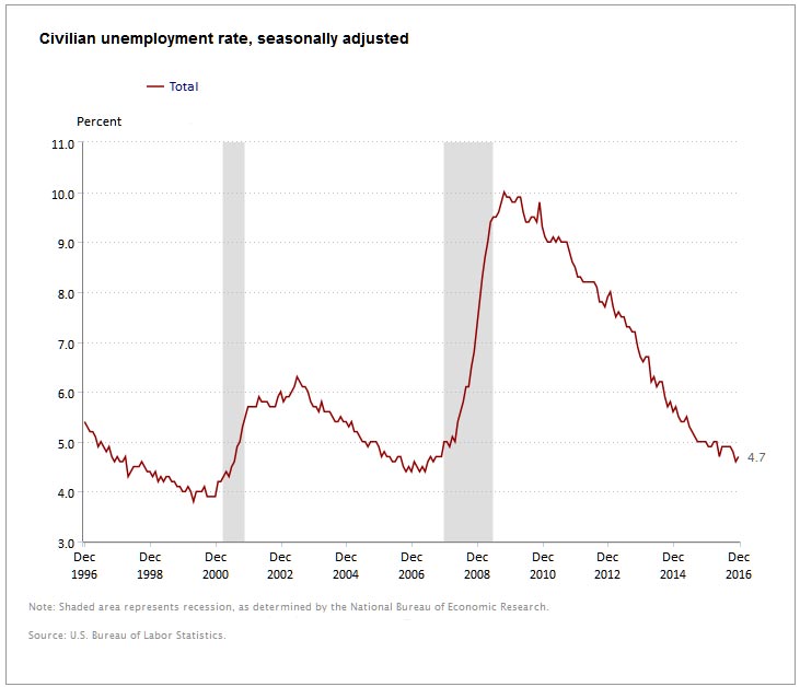
Now, it’s fair to say, the economy is near maximum employment and inflation is moving toward our goal. The unemployment rate is less than 5 percent, roughly back to where it was before the recession. And, over the past seven years, the economy has added about 15-1/2 million net new jobs. Although inflation has been running below our 2 percent objective for quite some time, we have seen it start inching back toward 2 percent last year as the job market continued to improve and as the effects of a big drop in oil prices faded. Last month, at our most recent meeting, we took account of the considerable progress the economy has made by modestly increasing our short-term interest rate target by 1/4 percentage point to a range of 1/2 to 3/4 percent. It was the second such step–the first came a year earlier–and reflects our confidence the economy will continue to improve.

Now, many of you would love to know exactly when the next rate increase is coming and how high rates will rise. The simple truth is, I can’t tell you because it will depend on how the economy actually evolves over coming months. The economy is vast and vastly complex, and its path can take surprising twists and turns. What I can tell you is what we expect–along with a very large caveat that our interest rate expectations will change as our outlook for the economy changes. That said, as of last month, I and most of my colleagues–the other members of the Fed Board in Washington and the presidents of the 12 regional Federal Reserve Banks–were expecting to increase our federal funds rate target a few times a year until, by the end of 2019, it is close to our estimate of its longer-run neutral rate of 3 percent.

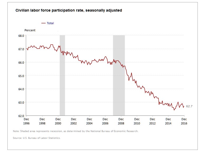
The term “neutral rate” requires some explaining. It is the rate that, once the economy has reached our objectives, will keep the economy on an even keel. It is neither pressing on the gas pedal to make the car go faster nor easing off so much that the car slows down. Right now our foot is still pressing on the gas pedal, though, as I noted, we have eased back a bit. Our foot remains on the pedal in part because we want to make sure the economic expansion remains strong enough to withstand an unexpected shock, given that we don’t have much room to cut interest rates. In addition, inflation is still running below our 2 percent objective, and, by some measures, there may still be some room for progress in the job market. For instance, wage growth has only recently begun to pick up and remains fairly low. A broader measure of unemployment isn’t quite back to its pre-recession level. It includes people who would like a job but have been too discouraged to look for one and people who are working part time but would rather work full time.

Nevertheless, as the economy approaches our objectives, it makes sense to gradually reduce the level of monetary policy support. Changes in monetary policy take time to work their way into the economy. Waiting too long to begin moving toward the neutral rate could risk a nasty surprise down the road–either too much inflation, financial instability, or both. In that scenario, we could be forced to raise interest rates rapidly, which in turn could push the economy into a new recession.

The factors I have just discussed are the usual sort that central bankers consider as economies move through a recovery. But a longer-term trend–slow productivity growth–helps explain why we don’t think dramatic interest rate increases are required to move our federal funds rate target back to neutral. Labor productivity–that is, the output of goods and services per hour of work–has increased by only about 1/2 percent a year, on average, over the past six years or so and only 1-1/4 percent a year over the past decade. That contrasts with the previous 30 years when productivity grew a bit more than 2 percent a year. This productivity slowdown matters enormously because Americans’ standard of living depends on productivity growth. With productivity growth of 2 percent a year, the average standard of living will double roughly every 35 years. That means our children can reasonably hope to be better off economically than we are now. But productivity growth of 1 percent a year means the average standard of living will double only every 70 years.

Economists do not fully understand the causes of the productivity slowdown. Some emphasize that technological progress and its diffusion throughout the economy seem to be slower over the past decade or so. Others look at college graduation rates, which have flattened out after rising rapidly in previous generations. And still others focus on a dramatic slowing in the creation of new businesses, which are often more innovative than established firms. While each of these factors has likely played a role in slowing productivity growth, the extent to which they will continue to do so is an open question.

Why does slow productivity growth, if it persists, imply a lower neutral interest rate? First, it implies that the economy’s usual rate of output growth, when employment is at its maximum and prices are stable, will be significantly slower than the post-World War II average. Slower economic growth, in turn, implies businesses will see less need to invest in expansion. And it implies families and individuals will feel the need to save more and spend less. Because interest rates are the mechanism that brings the supply of savings and the demand for investment funds into balance, more saving and less investment imply a lower neutral interest rate. Although we can’t directly measure the neutral interest rate, it is something that can be estimated in retrospect. And, as we have increasingly realized, it has probably been trending down for a while now. Our current 3 percent estimate of the longer-run neutral rate, for instance, is a full percentage point lower than our estimate just three years ago.

You might be thinking, what does this discussion of rather esoteric concepts such as the neutral rate mean to me? If you are a borrower, it means that, although the interest rates you pay on, say, your auto loan or mortgage or credit card likely will creep higher, they probably will not increase dramatically. Likewise, if you are a saver, the rates you earn could inch higher after a while, but probably not by a lot. For some years, I’ve heard from savers who want higher rates, and now I’m beginning to hear from borrowers who want lower rates. I can’t emphasize strongly enough, though, that we are not trying to help one of those groups at the expense of the other. We’re focused very much on that dual mandate I keep mentioning. At the end of the day, we all benefit from plentiful jobs and stable prices, whether we are savers or borrowers–and many of us, of course, are both.

Economics and monetary policy are, at best, inexact sciences. Figuring out what the neutral interest rate is and setting the right path toward it is not like setting the thermostat in a house: You can’t just set the temperature at 68 degrees and walk away. And, because changes in monetary policy affect the economy with long lags sometimes, we must base our decisions on our best forecasts of an uncertain future. Thus, we must continually reassess and adjust our policies based on what we learn.

Trump’s brand of Carrier-style dealmaking won’t work

From The Conversation.

In late November, President-elect Donald Trump announced that he had reached a deal with Carrier to keep about 800 manufacturing jobs in Indiana from moving to Mexico. After the announcement, we learned that the Indiana Economic Development Corporation would give US$7 million in tax credits and grants to Carrier’s parent company in exchange for keeping the jobs in the state.

Trump proudly praised the agreement as a “great deal for workers” and said that it was part of a larger approach to keep jobs at home, saying “this is the way it’s going to be.”

Having the chief executive of the United States negotiate individualized deals with corporations is certainly a new approach to economic policy nationally, though it is not without precedent. In fact, state governments have been negotiating targeted incentives with corporations for decades.

My research focuses on why states use incentives to attract and retain investment from corporations and whether they are effective. My work, as well as that of many others, shows that these deals do not create the jobs and economic growth they are purported to.

A common economic tool

Every year, states spend billions of dollars to entice companies to create jobs within their borders. These inducements include some combination of property, sales and income tax credits and rebates, tax abatements, cash grants and cost reimbursements.

The deals are meant to reduce costs for the businesses that receive them in order to encourage their investment and job growth in a particular location. The most prominent packages usually grab headlines nationally.

In 2013, for example, Boeing received $8.7 billion in tax breaks from Washington state to secure the production of the 777x. This record-breaking package came shortly after Boeing had received $900 million from South Carolina for opening a new 787 assembly plant in Charleston.

Other examples include Tesla receiving $1.3 billion from Nevada in 2014 to subsidize a battery factory outside Reno and the Los Angeles Rams collecting $180 million in sales tax revenue from Inglewood for relocating there from St. Louis this year.

Just as Carrier threatened to move jobs to Mexico and promptly received a tax break, so too did Sears receive millions from Illinois to keep its headquarters in Chicago back in 1989.

From 1984 to 2012, incentive spending increased in the states from about $500 million per year to about $13 billion per year, according spending data gathered by the Good Jobs First Subsidy Tracker.

Has it worked?

Despite the hundreds of billions of dollars in incentives thrown their way, many companies have still decided to move more manufacturing jobs and corporate headquarters overseas.

This is because corporations consider many other factors when making decisions about where to build a factory or establish a tax home. In a 2016 survey, incentives lagged behind skilled labor, labor costs, highway access, corporate tax rates, available buildings, construction costs, proximity to markets and quality of life as important factors for location decisions.

For example, scholars have found that the Sun Belt has been able to attract investment away from the Rust Belt because it has lower wages but similar access to the interstate highway system.

In other words, jobs move (or don’t) based on the overall range of costs facing employers, which are determined by larger economic trends and policies and not necessarily by individually negotiated deals. When subsidies do matter is when corporations are choosing between equally strong locations. In those situations, incentives serve as “deal sweeteners” but don’t change the fundamental reasons for why the location was considered in the first place.

In light of the realities of corporate location decisions, there is scant evidence to support the arguments that targeted incentives produce economic growth. Rather, the evidence shows that they tend to fail to achieve their intended goals.

Often, subsidies fall short of job creation targets and fail to create growth, even if they retain jobs. As University of Iowa scholars Alan Peters and Peter Fisher argue, based on a review of several studies of their impact, “incentives work about 10 percent of the time and are simply a waste of money the other 90 percent.”

One reason why scholars have struggled to measure the impact of incentives is because of the complexity of the economy. Economic growth is affected mostly by national and international forces. State economic development strategies have little effect when compared with broad national economic policies.

The wrong kind of impact

Subsidies still can have an effect on economic behavior, just not in the way they were intended, such as by encouraging rent-seeking.

Critics of the Carrier deal have already noted that Trump may have opened the federal government up to increased threats from companies to move overseas unless they receive more incentives (aka rent-seeking). In the days following the Carrier deal, Ford Motor (already one of the largest recipients of state-level spending) expressed a willingness to make a deal with Trump to retain jobs scheduled to move overseas. In a first move, Ford announced that it had canceled a planned investment in Mexico and will instead invest $700 million in its Flat Rock, Michigan, plant.

There is also some evidence that incentives can exacerbate economic inequality.

Incentives, when used to influence location decisions, tend to be awarded to the largest and wealthiest corporations. These corporations need the money the least of all businesses and usually receive the money for making investments they likely would have made anyway in order to remain competitive. The result is that fewer resources are available for education, workforce training and social services. As a result, the gap between rich and poor tends to grow.

Raising red flags

While it is laudable that several hundred Indianans get to celebrate the holiday season with their jobs secure, evidence from the states raises red flags on the viability of targeted incentives as a national policy for growth.

Not only would Trump be needing to negotiate several packages per week in order to have a noticeable effect on the U.S. economy, doing so opens the government up to increased demands for subsidies, most likely from the wealthiest corporations, and could exacerbate income inequality in America.

Author: Joshua Jansa, Assistant Professor of Political Science, Oklahoma State University

Have The U.S. Stock Bulls Got It Wrong?

From Bloomberg.

Amundi SA, Europe’s largest money manager, says investors who have driven U.S. stock markets to record highs in expectation of fiscal stimulus from the Trump administration may be in for a surprise.


While a pivot to government spending and tax cuts may prolong the economic expansion in the U.S., Republican lawmakers will insist that fiscal measures don’t push up the deficit, Didier Borowski, the Paris-based asset manager’s head of macroeconomics, said in an interview. Even if President-elect Donald Trump succeeds in delivering stimulus, it won’t have an impact before next year, he said.

“Following the vote for Trump, markets have reacted as if there were only upside risks,” Borowski said in an interview in Munich. “U.S. equity markets could go further into bubble territory as risks are becoming increasingly asymmetric. That would be an opportunity to reallocate funds to bond markets.”

Trump’s surprise victory in the U.S. presidential election in November has driven investors out of bonds and into equities, accelerating a massive flow of funds that some investors say may last for years and spell the end of the multi-decade rally in bonds. The value of global equities climbed to $68 trillion from about $65 trillion the day before the election. Bonds have lost about $2 trillion in that time.

Financial market observers and investors are split about the continuation of that trend, sometimes named the “great rotation” from bonds to stocks, with Charles Schwab Corp.’s chief global strategist Jeffrey Kleintop anticipating the it has years to run. Amundi, which is controlled by Credit Agricole SA, says a more likely scenario is that bonds may rebound because growth will probably continue at a slow pace.

“Global uncertainties are at an unprecedented level with Brexit, Trump and elections in Europe,” Borowski said, adding the biggest risk would be a trade war between the U.S. and China. “The bond market isn’t dead yet. There are many unpredictable risks still looming and that’s why we really doubt that bond yields can jump that much. Investors will keep an exposure to U.S. Treasuries as a safe haven.”

Investors may also return to Europe, once the outcome of elections removes political uncertainty in the region, he said.

“Some investors have stayed clear of Europe following Brexit,” Borowski said. “At some point in the coming months we will be reassured concerning the political risks in Europe, especially in France, where we don’t expect French National Front leader Marine Le Pen to be elected.”

Amundi was created in 2010 when Credit Agricole and Societe Generale SA combined their asset-management businesses. It went public in 2015 to fund its international expansion as Societe Generale sold its stake.

Amundi agreed in December to buy Pioneer Investments from Italy’s UniCredit SpA for about 3.5 billion euros ($3.7 billion) in cash, bringing assets to more than $1.3 trillion and making it the world’s eighth-largest asset manager.

US Mortgage Rates Add Stress for Millennial Homebuyers

Fitch Ratings says the recent rise in US interest rates adds another obstacle for millennials seeking to enter the housing market.

Based on our calculations, the rate increase means the average US millennial borrower now has lost 9% in mortgage capacity since the beginning of October 2016. This leaves more millennials out of what has historically been one of the most important wealth-creation mechanisms, and could contribute to long-term shifts in savings and consumption.

Mortgage rates nearly hit a two-year high during the week of Jan. 5, 2017 according to Freddie Mac. The interest rate on a 30-year mortgage at the beginning of October 2016 was 3.42%. Last week, the rate climbed to 4.20%. The maximum loan a homebuyer could afford in September 2016 was $120,000 (the current median mortgage for borrowers under 35 according to the Federal Survey of Consumer Finances), all else being equal, the size of that loan would have dropped to approximately $109,000 by last week.

Historically low rates have been one of the few factors that have helped young adults to buy homes. If rates continue to rise, particularly if the rise occurs rapidly over a short time period, this could add yet another obstacle to homeownership. Many first-time homebuyers have seen mortgage capacity eroded by tight loan underwriting standards, rising student loan payments, high rents and stagnant wages.

The growth in the cost of higher education outpaced consumer price inflation for several decades. This led to an increase in both the number of student loan borrowers and the average amount owed. The median student loan monthly payment in 2016 was $203, according to the Federal Reserve Bank of Cleveland.

Tight underwriting played a significant role. Banks remain vigilant over regulatory risk, repurchase risk and the increased cost of servicing of delinquent loans. This means FICO scores for conventional loans to first-time homebuyers remain notably above the 720-730 range level typical prior to the crisis, although the scores have begun trending back toward historical averages.

The stresses are reflected in the US homeownership rate and increases in the portion of millennials who live at home. The homeownership rate for under 35-year-olds experienced a large drop, declining to 35% in 2016, from 41% in 2000, according to the US Census Bureau. During this time, rental costs increased faster than the incomes millennials earn.

For younger Americans forced to defer or abandon plans to buy a first home, the long-term financial effect of missing out on home-equity creation could be significant. Long-lasting shifts in savings and consumption patterns, while difficult to isolate now, will likely emerge more prominently in the coming years. This could mean other long-run affects including downward pressure on durable goods consumption, urban population growth and a decline in affluence, translating into lower birth rates and less secure retirements.

Credit Looks for US to Realise Potential

Moody’s says today’s still underperforming US economy leaves plenty of room for significant improvement in 2017 without the unwanted side effect of significantly faster price inflation. The US economy may be far from realizing its full potential.

January 2017 marks the 91st month of the current economic recovery and yet the US economy’s rates of resource utilization leave considerable room for additional production. In terms of the latest three-month averages, only 75.2% of industrial capacity was in use, while payrolls approximated a relatively low 57.0% of the working-age population. When previous upturns were of similar vintage in October 1998 and June 1990, the industrial capacity utilization rate averaged 82.7% and payrolls averaged 59.9% of the working age population.

Will this be the first economic recovery since the 1930s where the capacity utilization rate’s moving three month average fails to reach the 80% mark, where the latter is typically associated with the sufficient utilization of potential industrial output? Thus far in the current upturn, this version of capacity utilization has risen no higher than the 78.6% of Q4-2014. Figure 1 indicates a good deal of room to grow for industrial capacity utilization and, thus, lends support to the possibility of faster than 3% real GDP growth. By comparison, real GDP has risen by only 1.8% annualized, on average, for the current recovery to date and not since 2005’s 3.3% has growth managed to reach 3% for an entire calendar year. (Figure 1.)

In a similar vein, late 2016’s relatively low ratio of jobs to the working-age population preserves the possibility of a fuller utilization of US labor resources that could supply a noticeably faster rate of economic growth. However, the recent absence of labor productivity growth limits the extent to which faster jobs growth can quicken economic growth. (Figure 2.)

Yes, late 2016’s comparatively low rates of resource utilization hint of considerable upside potential for US business activity. Nevertheless, whether such potential is realized depends on a far from assured quickening of expenditures. For one thing, the recent strengthening of the dollar exchange rate heightens the importance of an acceleration by US household spending, which requires improved prospects for employment income.

The critical role of household expenditures cannot be overemphasized. Regardless of the more favorable tax treatment of capital outlays, businesses are only likely to significantly increase their production capabilities if they are convinced of sufficiently profitable markets for new and existing products.

Thus, businesses are likely to heed the warning of slower household spending growth implicit in the dip by payrolls’ annual increase from Q1-2015’s cycle high of 2.2% to Q4-2016’s 1.6%. The last two times payrolls decelerated in a similar manner, recessions arrived within 18 months.

Jobs outlook suggests spreads are too thin

Corporate credit is now very much priced for faster economic growth that will require the fuller utilization of US productive resources. The correlation between the high-yield bond spread and the moving three-month average of payrolls’ monthly percent change is a strong 0.78. Fourth-quarter 2016’s average monthly increase by payrolls of 0.11% predicts a 531 bp midpoint for the high-yield bond spread.

Accordingly, January 11’s far thinner high-yield bond spread of 405 bp implicitly expects faster jobs growth. However, as inferred from the Blue Chip consensus expectation of a drop by payrolls’ average monthly increase from 2016’s 180,000 jobs to 2017’s 161,000 jobs, the high-yield spread may soon be closer to 500 bp than to 400 bp.

Unemployment rate overstates labor market tightness

As opposed to the unemployment rate, the ratio of payrolls to the working-age population may now be the better estimate of labor market utilization, owing to the current recovery’s large number of labor force dropouts. For example, when the unemployment rate previously first fell to Q4-2106’s 4.7% in March 2006 and November 1997, payrolls averaged 60.2% of the working age population, which was well above Q4-2016’s 57.0%.

As inferred from the unemployment rate’s statistical relationship with the ratio of payrolls to the working-age population since 1988, Q4-2016’s ratio of 57.0% is ordinarily accompanied by a jobless rate of 6.8%. Even after allowing for how an aging workforce exerts a downward bias to the ratio of payrolls to the working-age population, the 4.7% unemployment rate still probably overstates the degree of labor market tightening. (Figure 3.)

In addition to an atypically low labor force participation rate, the 4.7% unemployment rate overstates labor-market tightness because of a relatively high U6 unemployment, or under-employment, rate. When the jobless rate’s moving three-month average previously first fell to 4.7% in March 2006 and November 1997, the U6 under-employment rate averaged 8.4%, considerably lower than Q4-2016’s 9.3%.

Nevertheless, the US labor market is firming up, as seen in the yearly increase of the average hourly wage from the 2.5% of Q4-2015 to Q4-2016’s 2.7%. However, when the unemployment rate’s three-month average last fell to 4.7% in Q1-2006, average hourly earnings posted a comparable increase of 3.4%. During the previous cycle, the yearly increase of the average wage’s moving three-month average peaked at the 3.8% of Q3-2006. By the time the moving three-month averages of the jobless rate and the U6 under-employment rate bottomed simultaneously in May 2007 (at 4.4% and 8.1%, respectively), the average hourly wage’s annual increase had slowed to 3.4%.

Despite an earlier acceleration by the hourly wage’s moving yearlong average from the 2.0% of the span-ended September 2004 to the 3.7% of the span-ended March 2007, the annual rate of growth for the core PCE price index peaked at a relatively modest 2.4%. By comparison, the core PCE price index rose by 1.7% annually during the three-months-ended November 2016. The possibly unfinished strengthening of the dollar exchange rate will limit the upside for US price inflation and just might intensify the price deflation still afflicting a number of internationally traded goods.

Ratio of jobs to the working-age population outshines other possible inflation indicators

The market’s recent obsession with December’s 2.9% yearly jump by average hourly earnings may have been unwarranted. After all, the annual rate of core PCE price index inflation generated a meaningless correlation of 0.04 with the yearly percent change of the average hourly wage.

By contrast, the ratio of payrolls to the working-age population again offers useful insight regarding labor market tightness and inflation risk. Since 1992, the year-to-year percentage point change for the ratio of payrolls to the working-age population shows a correlation of 0.31 with the annual rate of core PCE price index inflation, where this and forthcoming comparisons employ moving three-month averages.

As far as predicting core PCE price index inflation, the ratio of jobs to the working-age population also outperforms both the unemployment and U6 under-employment rates. For example, the jobless rate and its year-to-year percentage point change showed weaker correlations of -0.22 and -0.24 with the annual rate of core PCE price index inflation, while the U6 under-employment rate posted comparably measured correlations of -0.23 and -0.22, respectively. Thus, expectations of a continued mild rise by the ratio of payrolls to the working-age population suggest only a limited upside for core PCE price index inflation.

Consensus views on employment and industrial production favor a continuation of the Great Underutilization. Unless payrolls zoom ahead of recent forecasts, the midpoint for fed funds may finish 2017 no higher than 1.125%, while the 10-year Treasury yield spends most of the year under 2.5%. Only if the demand for US output delivers a big enough upside surprise might a substantially fuller utilization of resources help make America great again.

US Housing Finance Agencies Will Benefit from Cut in FHA Mortgage Insurance Premiums

Moody’s says on Monday, the US Department of Housing and Urban Development (HUD) announced that the Federal Housing Administration (FHA) will reduce by 25 basis points insurance premiums that borrowers pay on single-family mortgages. The premium cut is credit positive for US state Housing Finance Agencies (HFAs) because it will make FHA-insured mortgage loans more affordable to borrowers and increase HFA loan originations. The premium reduction will apply to new loans closing on or after 27 January.

HFAs are charged with providing and increasing the supply of affordable housing in their respective states for first-time homebuyers. The FHA, unlike other mortgage insurance providers, insure loans with loan-to-value ratios of up to 97%, which is key to the HFA lending base, given that first-time homebuyers often have limited funds for down payments.

The 25-basis-point decrease in the FHA’s insurance premium, which we expect will save new homeowners as much as $500 a year, also increases the competitiveness of HFA mortgage products. A lower FHA cost will attract more borrowers and stimulate stronger FHA loan originations at a time when mortgage interest rates are rising. As of 30 June 2016, FHA mortgage insurance provided the biggest share of the insurance on HFA pools, constituting approximately 38% of Moody’s-rated HFA whole-loan mortgages (see Exhibit 1), compared with 17% of mortgages utilizing private mortgage insurance.

HFA portfolio performance will strengthen because more loans will benefit from FHA insurance coverage. FHA insurance offers the deepest level of protection against foreclosure losses relative to other mortgage insurers because they cover nearly 100% of the loan principal balance plus interest and foreclosure costs. Additionally, the FHA provides the strongest claims-paying ability relative to private mortgage insurers. Although private mortgage insurers maintain ratings of Baa1 to Ba1, FHA insurance is backed by the US government.

The reduced FHA premiums will also benefit HFA to-be-announced (TBA) loan sales, which are secondary market sales using the Ginnie Mae TBA market. All loans utilizing Ginnie Mae must have US government insurance, and the FHA provides a substantial share of this insurance. Higher TBA sales will increase in HFA margins given that TBA sales have been a major driver of loan production and volume, contributing to an all-time high 17% margin in fiscal 2015, which ended 30 June 2015 (see Exhibit 2).

Will the ‘Trump rally’ continue through 2017?

From The Conversation.

So far, investors appear to be giving Donald Trump their vote of confidence.

After his election as the 45th president of the United States, the U.S. Dollar Index rallied around 4 percent through the end of the year, while the Dow Jones Industrial Average approached 20,000 for the first time in its history and the Standard & Poor’s 500 was up just under 5 percent.

So now that investors have finished their usual year-end review of where to put their money, one question is on everyone’s mind: Will the so-called Trump rally continue in 2017?

In early November, I wrote an article based on my study showing that how stocks reacted in the first few days after a president’s victory would likely determine their performance for the rest of 2016 – which turned out to be true in Trump’s case.

In a similar vein, a separate study I published in 2009 demonstrated that how a stock market performs in the January a president takes office could portend its fortunes for the remainder of the year.

So will that also turn out to be true for Trump?

‘As January goes’

In that study, which I called “The ‘Other’ January Effect and the Presidential Election Cycle,” I combined two lines of research.

First, going at least as far back as the 1940s, the so-called January effect is a well-known bias in individual stock behavior in which stocks that lose value at the end of the year tend to reverse those losses in January.

The other January effect, which I use in my study, refers to evidence published in 2005 suggesting that January’s returns hold predictive power for the remainder of the year.

More specifically, this effect claims that when stocks go up in January, they tend to continue to climb for the rest of the year, and vice versa – regardless of the impact of other usual drivers of stock market returns. On Wall Street, this effect is often dubbed: “As January goes, so goes the year.” For the rest of the article, for simplicity’s sake, I’ll call this the January effect.

Second, I combined this January effect with the four-year presidential election cycle (PEC) to see how it influenced January’s predictive abilities. The PEC refers to a cycle in which U.S. stock market returns during the last two years of a president’s term tend to be significantly higher than gains during the first two years. This cycle is especially true for the third year of a president’s term, which has almost always been positive.

For my study, I wanted to see if the timing of the presidential cycle (first year, second year, etc.) affected January’s predictive abilities. I studied monthly returns (without dividends) of the S&P 500 over the 67-year period from 1940 through 2006.

January’s predictive power

Overall, my results were consistent with the paper noted above demonstrating that positive returns in January typically portended gains during the other 11 months of the year, as well as the opposite.

They further showed, however, that January’s predictive power is most convincing during the president’s first and fourth years in office. Since, at the moment, we care most about the first year of a president’s term, I’ll focus on those results.

Over my sample period of basically 17 election cycles, I found that during the president’s first year in office, average returns for the 11 months following a positive January were 12.29 percent, while a negative January led to average losses of 7.91 percent over the remainder of the year. That’s a difference of more than 20 percentage points – or over US$200,000 on a $1 million investment.

Furthermore, I found that a positive or negative January predicted returns for the remainder of the year almost 90 percent of the time, suggesting a very strong correlation.

Recent results have been split

Since my study was published, there have been two more elections, one of which ran contrary to the January effect, while the other confirmed it.

After President Barack Obama won the 2008 election, the S&P 500 lost 8.6 percent during his inaugural month of January. But the market rallied for the remainder of the year by about 35 percent.

Conversely, after his reelection in 2012, stocks returned around 5 percent in January 2013 and, consistent with the other January effect, the market climbed another 23 percent over the remainder of the year.

What’s behind this?

So what’s driving the effect?

Exactly what drives this effect is a topic of debate. For example, I tested whether it may be driven by monetary policy, which did not seem to be the case.

A common argument for the PEC is that it reflects investor views of fiscal policy, which is why returns during the second two years of the cycle tend to be higher than the first two. Yet my most significant results were for the first and fourth years.

Nonetheless, while I did not specifically test for fiscal policy influences, it seems valid since my results showed that January’s effect appears to be the most reliable during the president’s incoming year in office. The effect wasn’t nearly as pronounced during the other three years.

So far, that seems to be the case at the moment as the “Trump rally” appears to be a response to anticipated fiscal policy.

What to expect in 2017

Of course, there is never complete certainty in the markets, especially with an unavoidably small sample size like 17 election cycles. Still, the results of my study provide compelling evidence that, particularly in the president’s first year in office, January’s returns appear to capture information that is valuable for anticipating returns for the remainder of the year.

As of Jan. 10, the S&P 500 was up about 1.5 percent for the year and near its record high of 2,282, while the Dow continued to flirt with that magical 20,000 number.

While January’s full-month returns are not yet known, history strongly suggests that investors would be wise to closely monitor the S&P 500. If January 2017 remains positive for U.S. stocks, returns for the remainder of 2017 may very likely also be positive. The opposite can also be expected.

So for investors looking ahead in 2017, as January goes, perhaps so will the remainder of 2017.

Author: Ray Sturm, Associate Lecturer of Finance, University of Central Florida

How speeding up payments to small businesses creates jobs

From The US Conversation.

Speeding up payments to SME’s would have a major positive impact. Operating a small business, the backbone of the U.S. economy, has always been tough. The same is true in Australia, and cash flow is a major challenge, as data from our SME survey shows:

According to The Conversation, SME’s also been disproportionately hurt by the Great Recession, losing 40 percent more jobs than the rest of the private sector combined.

Interestingly, as my research with Harvard’s Ramana Nanda shows there’s a fairly straightforward way to support small businesses, make them more profitable and hire more: pay them faster.

A major source of financing

When a business is not paid for weeks after a sale, it is effectively providing short-term financing to its customers, something called “trade credit.” This is recorded in the balance sheet as accounts receivable.

Despite its economic importance, trade credit has received little attention in the academic literature so far, relative to other sources of financing, yet it is a major source of funding for the U.S. economy. The use of trade credit is recorded on companies’ accounting statements as “trade payables” in the liability section of the balance sheet. According to the Federal Fund Flows, trade payables amounted to US$2.1 trillion on nonfinancial companies’ balance sheets at the end of the third quarter of 2006, two times more than bank loans and three times as much as a short-term debt instrument known as commercial paper.

Recent news reports have highlighted the problem of slow payments to suppliers as large companies extend their payment periods, often with crushing results for small businesses.

Other countries have tried to reform the trade credit market, especially in Europe, where a directive was adopted in 2011 limiting intercompany payment periods for all sectors to 60 days (with a few exceptions).

In an earlier paper, I showed that requiring payments to be made within shorter time periods had a large effect on small businesses’ survival when it was adopted in France. Receiving their money earlier led them to default less often on their own suppliers and their financiers. Their probability to go bankrupt dropped by a quarter.

Accelerating payments

To learn more about the impact of such reforms in the U.S., we studied the effects of speeding up payments to federal contractors.

The QuickPay reform, announced in September 2011, accelerated payments from the federal government to a subset of small business contractors in the U.S., shrinking the payment period from 30 days to 15 days – thus accelerating $64 billion in annual federal contract value.

Federal government procurement amounts to 4 percent of U.S. gross domestic product and includes $100 billion in goods and services purchased directly from small businesses, spanning virtually every county and industry in the U.S. In the past, government contracts required payment one to two months following the approval of an invoice, with the result that these small businesses were effectively lending to the government – and often while doing so, they had to simultaneously borrow from banks to finance their payroll and working capital.

Our research shows that even small improvements in cash collection can have large direct effects on hiring due to the multiplier effect of working capital. On average, each accelerated dollar of payment led to an almost 10 cent increase in payroll, with two-thirds of the increase coming from new hires and the balance from increased earnings per worker. Collectively, the new policy – which accelerated $64 billion in payments – increased annual payroll by $6 billion and created just over 75,000 jobs in the three years following the reform.

To give an example, take a business selling $1 million throughout the year to its customers and being paid 30 days after delivering its product. It therefore has to finance 30 days’ worth of sales at any given time (or 8 percent of its annual sales). As a result, it constantly has about $80,000 in cash tied up in accounts receivable.

A shift in the payment regime from 30 days to 15 days means that the firm has to finance only 15 days of sales, or $40,000. And that would in turn help it eventually sustain $2 million in annual sales and double in size.

Holding back growth

These findings confirm the widely shared belief among policymakers and business owners that long payment terms hold back small business growth.

They also raise the question as to why the economy relies so much on trade credit if it costs so much in terms of jobs, and whether other policies might be undertaken to reduce it. An interesting follow-up policy to QuickPay was SupplierPay. In that program, over 40 companies including Apple, AT&T, CVS, Johnson & Johnson and Toyota pledged to pay their small suppliers faster or enable a financing solution that helps them access working capital at a lower cost.

It is likely that more information on customers’ quality and speed of payments would allow suppliers to choose whether to work with businesses that pay more slowly. So following a “name and shame” logic, companies might feel they have to accelerate payments not to be perceived as bad customers.

The broader impact

Would it make sense to sustain and extend this policy?

An interesting aspect of our analysis is that the effect of QuickPay depends on local labor market conditions. It was most pronounced in areas with high unemployment rates when it was introduced. Elsewhere job creation was limited.

The reason for this is that helping small businesses grow gives them an advantage over other companies operating locally. By hiring more, these small business contractors make it harder for others to do so. Unless there is unemployment, this crowding-out effect offsets the employment gains of the policy.

As such, such a policy will be effective in stimulating total employment only in areas or times of high unemployment.

Author: Jean-Noel Barrot, Assistant Professor of Finance, MIT Sloan School of Management

The Problem With Low Interest Rates

Fed Governor Jerome H. Powell spoke on “Low Interest Rates and the Financial System“. Monetary policy may sometimes face trade offs between macroeconomic objectives and financial stability. He argues that”low for long” interest rates have supported slow but steady progress to full employment and stable prices, which has in turn supported financial stability. But, there are difficult trade offs to manage. Over time, low rates can put pressure on the business models of financial institutions. And low rates can lead to excessive leverage and broadly unsustainable asset prices.

Whilst there are times when all of these objectives are aligned. For example, the Fed’s initial unconventional policies supported both market functioning and aggregate demand. More broadly, post-crisis monetary policy supported asset values, reduced interest payments, and increased both employment and income. All of these effects are likely to have limited defaults and foreclosures and bolstered the balance sheets of households, businesses, and financial intermediaries, leaving the system more robust.

But at times there will be tradeoffs. Low-for-long interest rates can have adverse effects on financial institutions and markets through a number of plausible channels.

After all, low interest rates are intended to encourage some risk-taking. The question is whether low rates have encouraged excessive risk-taking through the buildup of leverage or unsustainably high asset prices or through misallocation of capital. That question is particularly important today. Historically, recessions often occurred when the Fed tightened to control inflation. More recently, with inflation under control, overheating has shown up in the form of financial excess. Core PCE inflation remained close to or below 2 percent during both the late-1990s stock market bubble and the mid-2000s housing bubble that led to the financial crisis. Real short- and long-term rates were relatively high in the late-1990s, so financial excess can also arise without a low-rate environment. Nonetheless, the current extended period of very low nominal rates calls for a high degree of vigilance against the buildup of risks to the stability of the financial system.If we look at the channels listed here, the picture is mixed, but the bottom line is that there has not been an excessive buildup of leverage, maturity transformation, or broadly unsustainable asset prices.

Low long-term interest rates have weighed on profitability in the financial sector, although firms have so far coped with those pressures. Net interest margins (NIMs) for most banks have held up surprisingly well. NIMs have moved down for the largest banks
Return on assets, has recovered but remains below pre-crisis levels. Life insurers have substantially underperformed the broader equity market since 2007, suggesting that investors see the low-rate environment as a drag on profitability for the industry. Even so, data on asset portfolios do not suggest that life insurers have increased risk-taking. The same is true for banks. Both the regulatory environment and banks’ own attitudes toward risk following the financial crisis have helped ensure that the largest banks have not taken on excessive credit or duration risks relative to their capital cushions.

Low rates have provided support for asset valuations–indeed, that is part of their design. But I do not see valuations as significantly out of line with historical experience. Equity prices have recently increased considerably, pushing the forward price-earnings ratio further above its historical median.

And equity premiums –the expected return above the risk-free rate for taking equity risk– have declined, but are not out of line with historical experience.

In the nonfinancial sector, valuation pressures are most concerning when leverage is high, particularly in real estate markets. Residential real estate valuations have been in line with rents and household incomes in recent years, and the ratio of mortgage debt to income is well below its pre-crisis peak and still declining. In contrast, valuations in commercial real estate are high in some markets. And in the nonfinancial corporate sector, gross leverage is high by historical standards. Low long-term rates have encouraged corporate debt issuance at the same time that some regulations, particularly the Volcker rule, have discouraged banks from holding and making markets in such debt. High-risk corporate debt (the sum of high-yield bonds and leveraged loans) grew rapidly in 2013 and 2014, although growth has declined sharply since then.

However, firms also are holding high levels of liquid assets, so net leverage is not elevated. Firms have also lengthened their maturity profiles, and interest coverage ratios are high. Greenwood and Hanson’s measure of the share of high-yield debt in overall issuance is at a relatively low level. And this debt is now held more by unlevered investors. Overall, I do not see leveraged finance markets as posing undue financial stability risks. And if risk-taking does not threaten financial stability, it is not the Fed’s job to stop people from losing (or making) money.

As I said, a mixed picture. Low interest rates have encouraged risk-taking and higher leverage in some sectors and have weighed on profitability in others, but the areas where there are signs of excess are isolated.

US Employment Data Strengthens Case For More Rate Rises

The latest US Bureau of Labor Statistics, released overnight shows US employment momentum is supportive of rate rises this year. It is ironic that as the US presidency passes in a couple of week, the economy there is looking pretty strong! Over the past 3 months, job gains have averaged 165,000 per month. However the news was not sufficient to lift the Dow Index through 20,000.

Household Survey Data

The unemployment rate, at 4.7 percent, and the number of unemployed persons, at 7.5 million, changed little in December. However, both measures edged down in the fourth quarter, after showing little net change earlier in the year.

Among the major worker groups, the unemployment rates for adult men (4.4 percent), adult women (4.3 percent), teenagers (14.7 percent), Whites (4.3 percent), Blacks (7.8 percent), Asians (2.6 percent), and Hispanics (5.9 percent) showed little change in December.

The number of long-term unemployed (those jobless for 27 weeks or more) was essentially unchanged at 1.8 million in December and accounted for 24.2 percent of the unemployed. In 2016, the number of long-term unemployed declined by 263,000.

The labor force participation rate, at 62.7 percent, changed little in December and was unchanged over the year. In December, the employment-population ratio was 59.7 percent for the third consecutive month; this measure showed little change, on net, in 2016.

The number of persons employed part time for economic reasons (also referred to as involuntary part-time workers), at 5.6 million, was essentially unchanged in December but was down by 459,000 over the year. These individuals, who would have preferred full-time employment, were working part time because their hours had been cut back or because they were unable to find a full-time job.

In December, 1.7 million persons were marginally attached to the labor force, little changed from a year earlier. (The data are not seasonally adjusted.) These individuals were not in the labor force, wanted and were available for work, and had looked for a job sometime in the prior 12 months. They were not counted as unemployed because they had not searched for work in the 4 weeks preceding the survey.

Among the marginally attached, there were 426,000 discouraged workers in December, down by 237,000 from a year earlier. (The data are not seasonally adjusted.) Discouraged workers are persons not currently looking for work because they believe no jobs are available to them. The remaining 1.3 million persons marginally attached to the labor force in December had not searched for work for reasons such as school attendance or family responsibilities.

Establishment Survey Data

Total nonfarm payroll employment rose by 156,000 in December, with an increase in health care and social assistance. Job growth totaled 2.2 million in 2016, less than the increase of 2.7 million in 2015.

Employment in health care rose by 43,000 in December, with most of the increase occurring in ambulatory health care services (+30,000) and hospitals (+11,000). Health care added an average of 35,000 jobs per month in 2016, roughly in line with the average monthly gain of 39,000 in 2015.

Social assistance added 20,000 jobs in December, reflecting job growth in individual and family services (+21,000). In 2016, social assistance added 92,000 jobs, down from an increase of 162,000 in 2015.

Employment in food services and drinking places continued to trend up in December (+30,000). This industry added 247,000 jobs in 2016, fewer than the 359,000 jobs gained in 2015.

Employment also continued to trend up in transportation and warehousing in December (+15,000). Within the industry, employment expanded by 12,000 in couriers and messengers. In 2016, transportation and warehousing added 62,000 jobs, down from a gain of 110,000 jobs in 2015.

Employment in financial activities continued on an upward trend in December (+13,000). This is in line with the average monthly gains for the industry over the past 2 years.

In December, employment edged up in manufacturing (+17,000), with a gain of 15,000 in the durable goods component. However, since reaching a recent peak in January, manufacturing employment has declined by 63,000.

Employment in professional and business services was little changed in December (+15,000), following an increase of 65,000 in November. The industry added 522,000 jobs in 2016.

Employment in other major industries, including mining, construction, wholesale trade, retail trade, information, and government, changed little in December.

The average workweek for all employees on private nonfarm payrolls was unchanged at 34.3 hours in December. In manufacturing, the workweek edged up by 0.1 hour to 40.7 hours, and overtime edged up by 0.1 hour to 3.3 hours. The average workweek for production and nonsupervisory employees on private nonfarm payrolls remained at 33.6 hours.

In December, average hourly earnings for all employees on private nonfarm payrolls increased by 10 cents to $26.00, after edging down by 2 cents in November. Over the year, average hourly earnings have risen by 2.9 percent. In December, average hourly earnings of private-sector production and nonsupervisory employees increased by 7 cents to $21.80.

The change in total nonfarm payroll employment for October was revised down from +142,000 to +135,000, and the change for November was revised up from +178,000 to +204,000. With these revisions, employment gains in October and November were 19,000 higher than previously reported. Over the past 3 months, job gains have averaged 165,000 per month.