The fall in interest rates and an easing of lending standards will “breathe life” into the property market, but not without consequences, according to Moody’s Analytics, via The Adviser.
Financial intelligence agency Moody’s Analytics has released its Second Quarter 2019 Housing Forecast Report, in which it has noted its outlook for the Australian housing market.
Drawing on CoreLogic’s Hedonic Home Value Index,
the research agency noted the correction in residential property
prices, which it said was “a long time coming” after a “strong run-up”
in values across more densely populated markets, particularly in Sydney
and Melbourne.
However, Moody’s has observed that while
residential home prices have moderated from their peak in September
2017, the decline has not led to a “material” improvement in housing
affordability, with values still 20 per cent higher than during the
pre-boom period in 2013.
Nonetheless, Moody’s has reported that it expects the Reserve Bank of Australia’s (RBA) cut to the official cash rate and proposals
to ease home loan serviceability guidelines from the Australian
Prudential Regulation Authority (APRA) to rekindle demand for credit and
spark activity in the housing market.
“An important driver of the
slowdown in Australia’s housing market has been tighter credit
availability, partly as a consequence of the regulator – the Australian
Prudential Regulation Authority – tightening lending conditions, which
has made it relatively more difficult to purchase a property,
particularly for investors,” Moody’s noted.
“These serviceability requirements were eased in May.
“Expectations
of further lending reductions flowing on from RBA cash rate reductions
will also breathe life into the property market and add weight to our
view that the national housing market will reach a trough in the third
quarter of 2019 and gradually improve thereafter.”
However,
Moody’s warned that a resurgence in the housing market activity could
further expose the economy to risks associated with high levels of
household debt.
“This could see the household leverage-to-GDP
ratio climb, making Australia stand out further amongst its peers,”
Moody’s stated.
“This is an undesirable position to be in,
particularly given the questions around sustainability of the
potentially rising debt load.”
Moreover, recent changes in the
regulatory landscape have been interpreted by some observers as as a
sign that the economy could be at risk of falling into recession amid growing internal and external headwinds.
Treasurer Josh Frydenberg recently acknowledged that “international challenges” could pose a threat to the domestic economy.
Fears
of a looming recession have prompted some observers, including the CEO
of neobank Xinja, Eric Wilson, to encourage borrowers to pocket mortgage rate cuts passed on following the RBA’s decision to lower the cash rate.
Mr
Wilson claimed that resisting the urge to accrue more debt would help
borrowers build a buffer against downside risks in the economy.
The
Australian Bureau of Statistics’ (ABS) Australian National Accounts
data for the quarter ending March 2019, reported GDP growth of 0.4 per
cent, with annual growth slowing to 1.8 per cent – the weakest since
September 2009.
However, Moody’s economist Katrina Ell has said she expects the RBA’s monetary policy agenda to help revive the economy.
“The
combination of increased monetary policy stimulus, expectations of the
housing market reaching a trough in the third quarter of 2019, and
fiscal policy playing a relatively supportive role including via income
tax cuts should boost GDP growth to 2.8 per cent in 2020,” Ms Ell said.
In the Phase 2 document released today, Deposit Insurance, funded by a bank levy is proposed. Unlike the Australian $250k scheme (which is not activated until the Government says so, and is taxpayer funded initially), the NZ scheme is for a lower amount with a protection limit in the range of $30,000 – $50,000. Implementation will probably take at least two years.
One question so far not answered is the interaction with the deposit bail-in. Generally bail-in stops a failing bank from failing, whereas deposit guarantees are activated on failure. So bail-in might stop deposit guarantees even being called on…
Depositor Protection
Why is a range of $30,000 – $50,000 for the proposed depositor protection scheme proposed?
Available data suggests that a protection limit in the range of
$30,000 – $50,000 could fully protect from loss more than 90 percent of
individual bank depositors in New Zealand, while leaving the majority of
banks’ deposit funding exposed to risk. This would strike the right
balance between protecting small depositors from loss and enhancing
public confidence in the banking system on the one hand, while
maintaining private incentives to monitor bank risk taking on the other.
It would also be broadly consistent with international schemes in terms
of the share of deposits and depositors that would be fully protected
(albeit relatively low in terms of the absolute dollar value of
protections).
More work will be required to choose the limit within this range that
is the best for advancing the public policy objectives chosen for the
protection scheme. The consultation seeks feedback on these choices.
The Reserve Bank is proposing high capital requirements for
banks which should reduce the risk of bank failure. Why is depositor
protection required if the risk of bank failure is small?
Even with high capital requirements, banks can still fail for a
variety of reasons. Regulation, supervision, resolution, and deposit
protection all make up a ‘financial safety net’ that supports a stable
and resilient financial system and protects society from the damage
caused by bank failures. The safety net tools interact and overlap,
which can make it seem that not all of the tools are necessary. However,
if the safety net is incomplete, it will be difficult to find effective
solutions for dealing with serious problems in the banking system. This
means that capital tools that help to keep banks safe and sound at the
‘top of the cliff’, must be complemented by robust tools to deal with
banks that may still fall to the bottom.
The OECD and IMF have warned that, without depositor protection, New
Zealand is vulnerable to contagious bank runs. Bank runs can escalate
into banking crises that destroy social and financial capital. For New
Zealand’s safety net to be effective in good times and bad, the tools
within the net must each be strong in its own right, and work well
together.
How will the risks associated with moral hazard be addressed in the proposed depositor protection scheme?
Moral hazard arises when people are protected from the consequences
of their risky behaviour. If deposit protection is introduced,
depositors may take less care when assessing the risks associated with
their banks, and banks may take less care with depositors’ money. Moral
hazard costs are part of the reason why New Zealand has until now chosen
not to have a depositor protection regime.
There is considerable international experience on how to design an
effective deposit protection scheme, within the broader financial safety
net, that mitigates moral hazard. International experience demonstrates
that strong regulatory monitoring of deposit-takers’ corporate
governance and risk management systems goes a long way to addressing the
moral hazard of depositor protection. Maintaining private monitoring
incentives is also important, and can be achieved through carefully
calibrating the protection scheme’s scope of coverage. For example,
setting the protection limit at a level that fully covers most household
and small business depositors, but leaves large institutional
depositors exposed to risk, will support private monitoring incentives.
In conjunction, having effective resolution tools (that make it more
credible investors’ money is at risk should their institution fail) can
sharpen monitoring by institutional investors.
International practice and guidance, as well as the views of experts
and the public, will inform the design of New Zealand’s depositor
protection scheme.
What are the costs of funding the proposed depositor protection scheme and who will bear these costs?
A primary tool of the protection scheme will be insurance. Deposit
insurance transfers the risks and costs of bank failures away from
depositors onto an insurance scheme. This will come with upfront costs
of establishing a deposit insurer, and ongoing operational costs.
Modern deposit insurance schemes are normally funded by levies on
member banks, supported (where necessary) by temporary lending paid for
by taxpayers. If the insurance scheme is accompanied by a depositor
preference, this might also increase banks’ non-deposit funding costs as
risks are transferred from depositors onto institutional investors.
Details of the scheme, including costs, are still to be worked out in
the next phase of the work programme. To the extent that depositor
protection increases banks’ average costs, this might be passed on to
customers through higher mortgage rates or lower deposit rates.
Alternatively, costs might be absorbed by banks’ own margins and
retained earnings. The extent to which costs are shared between banks
and their customers depends on competition and contestability in the
sector.
A fuller cost-benefit analysis will follow as we learn more about the
specific design features of New Zealand’s depositor protection scheme.
When will the depositor protection scheme be introduced?
A work programme running alongside the Reserve Bank Review process
will develop a depositor protection scheme that is best for New Zealand.
The work programme will be guided by a framework setting out some key
design principles for an effective scheme, and will draw (where
relevant) on international standards and best practice. The work
programme will determine the:
mandates and powers
governance and decision making structure
coordination arrangements with other safety net providers
membership and coverage arrangements
funding and pay-out mechanics, and
design features to mitigate moral hazard
that are appropriate for New Zealand’s protection scheme. The Review
Team’s discussions with the global coordinating body for deposit
insurers indicates that the path from policy recommendations to scheme
implementation will probably take at least two years.
On 21 June, the US Federal Reserve (Fed) published the results of the 2019 Dodd-Frank Act stress test (DFAST) for 18 of the largest US banking groups, all of which exceeded the required minimum capital and leverage ratios under the Fed’s severely adverse stress scenario; via Moodys’.
These results are credit positive for the banks because they show that the firms are able to withstand severe stress while continuing to lend to the economy. In addition, most firms achieved a wider capital buffer above the required minimum than in last year’s test, indicating a higher degree of resilience to stress. The 2019 results support our view of the sector’s good capitalization and benefit banks’ creditors.
The median stressed capital buffer above the required Common Equity Tier 1 (CET1) ratio increased to 5.1% from 3.5% last year, a substantial change. However, the 18 firms participating in 2019 were far fewer than the 35 that participated in 2018, helping lift the results this year. This is because passage of the Economic Growth, Regulatory Relief, and Consumer Protection Act in May 2018 resulted in an extension of the stress test cycle to two years for 17 large and non-complex US bank holding companies, generally those with $100-$250 billion of consolidated assets, which pose less systemic risk.
This is the fifth consecutive year that all tested firms exceeded the Fed test’s minimum CET1 capital requirement. As in prior years, the banks’ Tier 1 leverage and supplementary leverage ratios had the slimmest buffers of 2.8% and 2.4%, respectively, above the required minimums as measured by the aggregate.
Under DFAST, the Fed applies three scenarios – baseline, adverse and severely adverse – which provide a forward-looking assessment of capital sufficiency using standard assumptions across all firms. The Fed uses a standardized set of capital action assumptions, including common dividend payments at the same rate as the previous year and no share repurchases. In this report, we focus on the severely adverse scenario, which is characterized by a severe global recession accompanied by a period of heightened stress in commercial real estate markets and corporate debt markets.
This year’s severely adverse scenario incorporates a more pronounced economic recession and a greater increase in US unemployment than the 2018 scenario. The 2019 test assumes an 8% peak-to-trough decline in US real gross domestic product compared with 7.5% last year and a peak unemployment rate of 10% that, although the same as last year, equates to a greater shock because the starting point is now lower (the rise to peak is now 6.2% compared with 5.9% last year).
The severely adverse scenario also includes some assumptions that are milder than last year: housing prices drop 25% and commercial real estate prices drop 35%, compared with 30% and 40% last year; equity prices drop 50% compared with 65% last year; and the peak investment grade credit spread is 550 basis points (bp), down from 575 bp last year. We consider this exercise a robust health check of these banks’ capital resilience.
Finally, the three-month and 10-year Treasury yields both fall in this year’s severely adverse scenario, resulting in a mild steepening of the yield curve because the 10-year yield falls by less. As a result banks’ net interest income faces greater stress than in last year’s scenario, which assumed unchanged treasury yields and a much steeper yield curve.
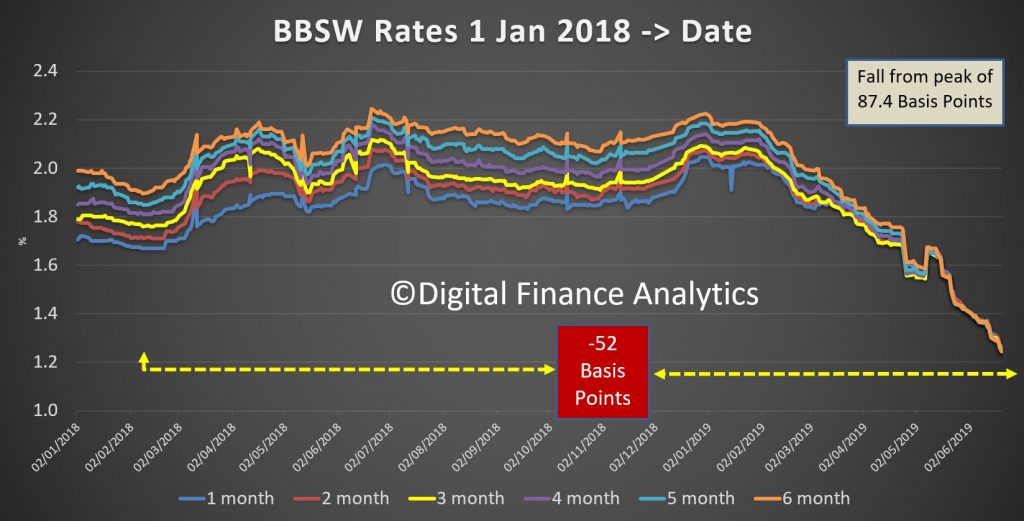
In the June RBA Bulletin, there was an article which describes how the RBA executes its market interventions to effect a cash rate change. It is important to understand these inner workings, despite it appearing complicated on first blush.
And consider this, this tool box is being used by many central banks around the world to direct the financial system.
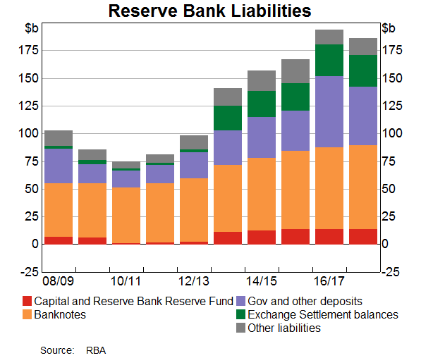
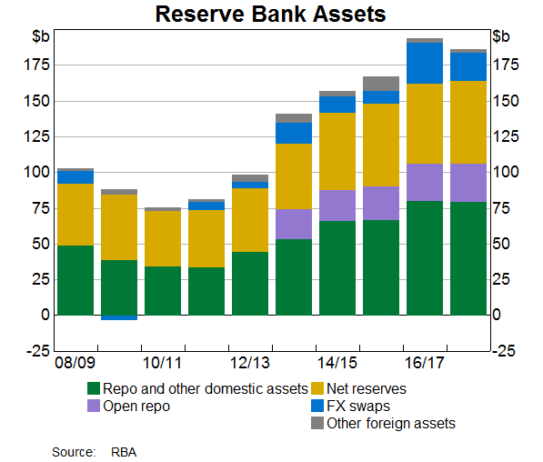
In summary, the RBA’s operations in domestic markets support the implementation of monetary policy. The most important tool to guide the cash rate to the target set by the Board is the interest rate corridor. To support this, the RBA pursues daily open market operations in order to keep the pool of exchange settlement (ES) balances at the appropriate level for the cash market to function smoothly. The daily market operations are conducted to offset the effects on liquidity of the many transactions between the banking system and the Australian Government. Open market operations are primarily conducted through repos and FX swaps. These provide flexibility for liquidity management and also help to manage risk for the RBA’s balance sheet.
The cash rate is a key determinant of interest rates in domestic financial markets and hence underpins the structure of the interest rates that influence economic activity and financial conditions more generally.
This helps to explain the sharp falls in the BBSW rates, which are now around 87 basis points lower than the recent peak. Such a fall has been engineered.
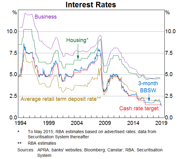
The cash rate is an effective instrument for implementing monetary policy because it affects the broader interest rate structure in the domestic financial system. The cash rate is an important determinant of short-term money market rates, such as the bank bill swap rate (BBSW), and retail deposit rates (Graph 1). These rates – as well as a number of other factors – then influence the funding costs of financial institutions and the lending rates faced by households and businesses. As a result, the cash rate influences economic activity and inflation, enabling the RBA to achieve its monetary policy objectives. However, while changes in the cash rate are very important, they are not the only determinant of market-based interest rates. Other factors, such as expectations, conditions in financial markets, changes in competition and risks associated with different types of loans are also important.
Graph 1
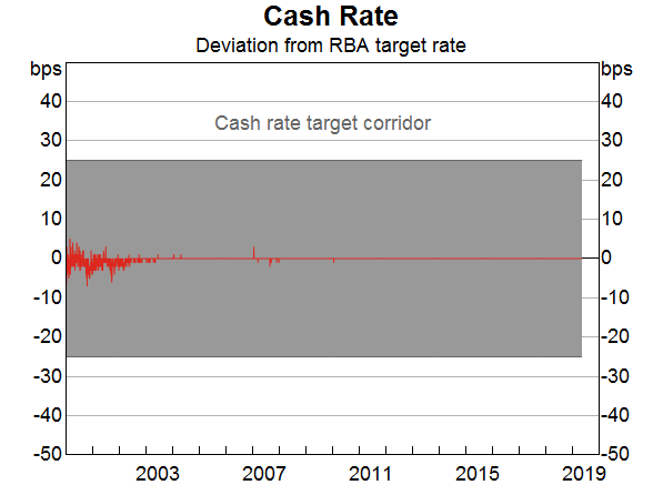
The Cash Market and the Interest Rate Corridor
The RBA implements monetary policy by setting a target for the cash rate. This is the interest rate at which banks lend to each other on an overnight unsecured basis, using the exchange settlement (ES) balances they hold with the RBA. ES balances are at-call deposits with the RBA that banks use to settle their payment obligations with other banks. Banks are required to have a positive (or zero) ES balance at all times, including at the end of each day. It is difficult for institutions to predict whether they will have adequate funds at the end of any particular day, which generates the need for an interbank overnight cash market. Those banks that need additional ES balances after they have settled all payment obligations of their customers, borrow from banks with surplus ES balances. The interbank cash market is the mechanism through which these balances are redistributed between participants.
The RBA sets the supply of ES balances to ensure that the cash market functions smoothly by
providing an appropriate level of ES balances to facilitate the settlement of interbank
payments. The RBA manages the supply of ES balances available to the financial system through
its open market operations (see below). Excessive ES balances could lead institutions to lend
below the target cash rate, while a shortage might result in the cash rate being bid up above
the target.
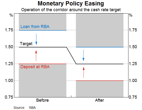
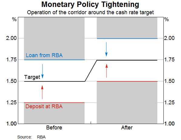
The interest rate corridor ensures that banks have no incentive to deviate significantly from
the cash rate target when borrowing or lending in the cash market. Banks can borrow ES balances
overnight on a secured basis from the RBA at a margin set 25 basis points above the cash rate
target. As a result, banks have no need to borrow from other banks at a higher rate. Similarly,
banks receive interest on their surplus ES balances at 25 basis points below the cash rate
target. Therefore, they have no incentive to lend to other banks at a lower rate.
The operation of the interest rate corridor means that there is no need for the RBA to adjust
the supply of ES balances to bring about a change in the cash rate (Graph 2 and Graph 3). For
example, when the RBA lowered the cash rate target by 25 basis points from 1.5 per cent
to 1.25 per cent in early June, the rates associated with the corridor also moved
lower, to be 1.0 per cent on overnight deposits and 1.5 per cent on
overnight loans (down from 1.25 per cent and 1.75 per cent). A bank that
would have previously required a return above 1.25 per cent to lend ES balances in the
cash market is, under the new corridor, willing to lend at a lower return. And so a bank wanting
to borrow cash pays a lower rate than before. Similarly, if the RBA had instead raised
the cash rate by 25 basis points from 1.5 per cent, the corridor would have moved up,
to be 1.5 per cent to 2.0 per cent. A bank that would have previously lent
surplus ES funds to another in the cash market at 1.50 per cent would, under the new
corridor, no longer have an incentive to do so. Indeed, it would require a higher return to lend
ES balances, rather than leaving those funds in its ES account and receiving 1.50 per cent
from the RBA. Hence, a bank wanting to borrow in the cash market would have to pay a higher
interest rate than it did previously.
In other words, interbank transactions automatically occur within the interest rate corridor without the RBA needing to undertake transactions beyond its usual market operations to manage liquidity.
Graph 2
Graph 3
The incentives underlying the corridor guide the cash rate to the target and ordinarily all transactions occur at the rate announced by the RBA. The last time there was a small deviation in the published cash rate (which is a weighted average of all transactions in the cash market) from the target (of 1 basis point for two days) was in January 2010 (Graph 4). The lack of deviation of the cash rate from the target has brought about a self-reinforcing market convention where both borrowers and lenders in the cash market expect to transact at the prevailing target rate. This market convention helps to address the uncertainty that banks would otherwise face about the price at which they can borrow sufficient ES balances to cover their payment obligations each day. In 2018, daily transactions in the overnight interbank market were typically between $3 billion and $6 billion.
Graph 4
As in Australia, many other central banks implement monetary policy with an interest rate corridor to guide the policy rate. The width of the corridor tends to differ, typically from 50 to 200 basis points. The choice of the width of the corridor is seen as a reflection of a trade‐off between interest rate control and the desire to avoid the central bank becoming an intermediary in the money market. All other things being equal, cross-country studies suggest that a narrower corridor is preferred by central banks that have a strong preference for low volatility of short-term interest rates, whereas a wider corridor is usually preferred by central banks that seek to encourage more interbank trading activity.
Over the past 10 years, many central banks (other than the RBA) have significantly expanded
their balance sheets. This has resulted in significantly more liquidity in their respective
systems and so banks typically do not need to borrow funds in the overnight cash market. In
these cases, the policy rate typically converges toward the rate on deposits paid by the central
bank; this is often referred to as a ‘floor system’. Small changes in liquidity in
such a system do not tend to have much effect on the policy rate.
Liquidity Management and Open Market Operations
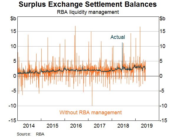
Transactions between the government (which banks with the RBA) and the commercial banks would, by themselves, change the supply of ES balances on a daily basis. ES balances in accounts of commercial banks increase whenever the government spends out of its accounts at the RBA. Similarly, when the government receives cash into its accounts at the RBA, such as from tax payments or debt issuance, ES balances decline. The RBA monitors and forecasts these changes actively through the day. It offsets (i.e. ‘sterilises’) these changes in ES balances with its daily open market operations so that government receipts and payments do not affect the aggregate level of ES balances. If transactions that affect system liquidity were not offset by the RBA, ES balances would be much more volatile and the payments system would suffer frequent disruptions (Graph 5). Ultimately this is likely to lead to a more volatile cash rate.
Graph 5
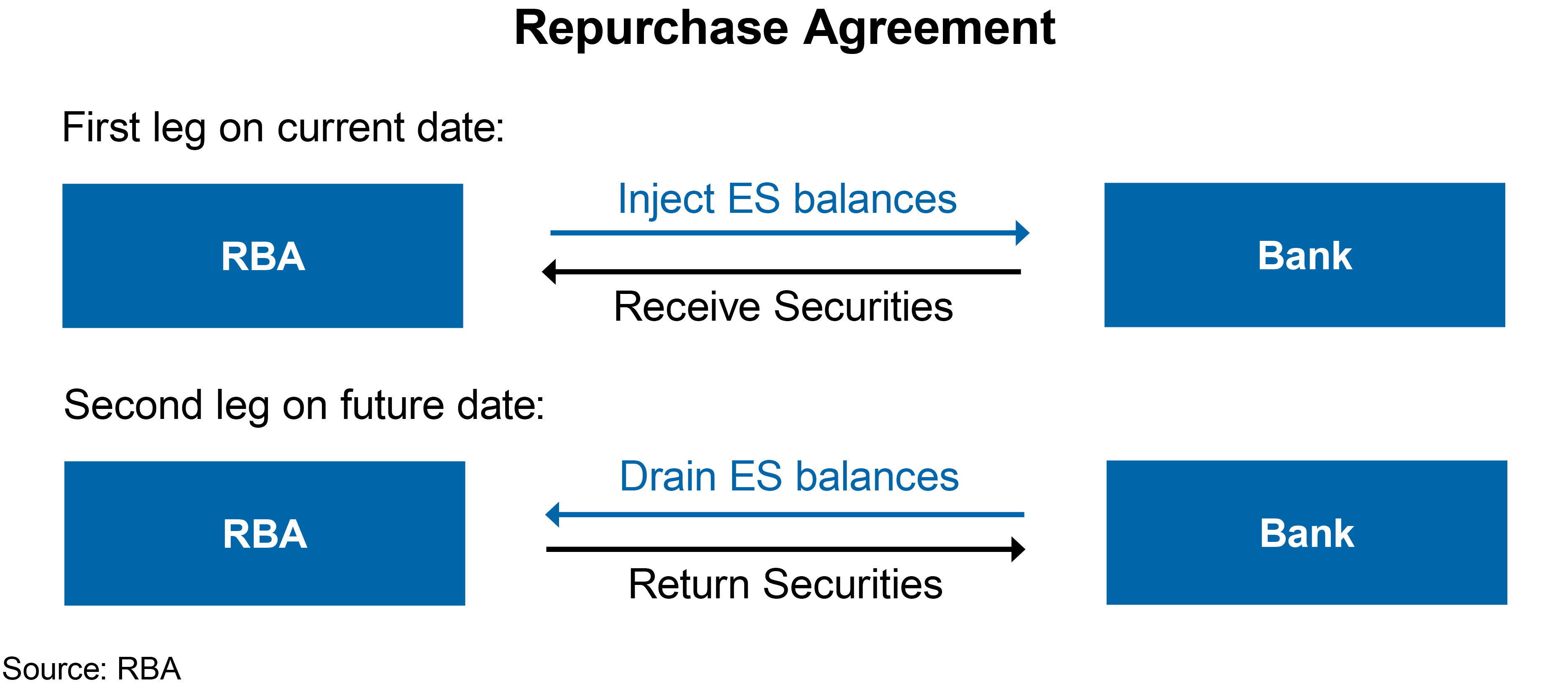
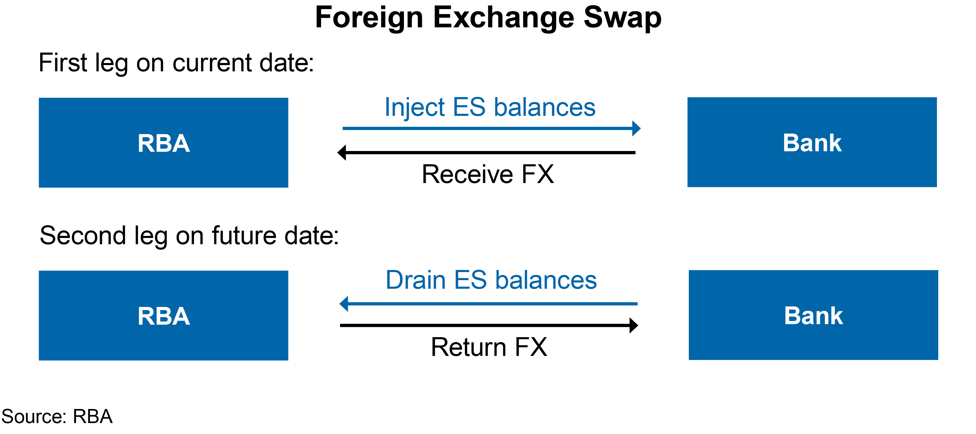
The main tools used in open market operations are repurchase (repo) agreements and foreign exchange swaps. Both repos and foreign exchange swaps involve a first and a second leg (Figures 1 and 2):
The first leg of a typical repo in open market operations (which injects ES balances)
involves the RBA providing ES balances to a bank and the bank providing eligible debt
securities as collateral to the RBA. Taking collateral safeguards the RBA against loss in
the case of counterparty default. The second leg, which occurs at an agreed future date,
unwinds the first leg: the bank returns the ES balances and the RBA returns the securities
to the bank.
The first leg of a foreign exchange swap designed to inject ES balances into the system
involves the RBA providing ES balances to a bank and the bank providing collateral in the
form of foreign currency to the RBA (typically US dollars, euros or Japanese yen). The
second leg, at the agreed future date, consists of the bank returning the ES balances and
the RBA returning the foreign exchange.
Figure 1
Figure 2
Repos and swaps provide more flexibility for liquidity management than outright purchases or sales of assets since they involve a second leg (when the transaction unwinds) with a date chosen to support liquidity management on that day. It also allows the RBA to accept a much broader range of collateral, such as unsecured bank paper, than it would be willing to purchase outright. By contrast, buying (and then selling) securities outright requires the RBA to take on the price and liquidity risk associated with owning the assets outright. Conducting open market operations by buying and selling government securities outright, while also ensuring that the RBA’s market operations do not affect liquidity in the bond market, would require more government securities than are available in Australia.
The size of daily open market operations is based on forecasts of daily liquidity flows between
the RBA’s clients (mainly the Australian Government) and the institutions with ES accounts.
In a typical round of market operations, a public announcement is made at 9.20 am that the RBA
is willing to auction ES balances against eligible collateral for a certain number of days
(ranging from two days to several months, with an average term of around 30 days). Institutions
have 15 minutes to submit their bid. The RBA ranks these bids from highest to lowest repo
rate and then allocates ES balances to the highest bidders until the amount the RBA intends to
auction has been dealt. All auction participants are informed electronically about their
allocation. If they have been successful, they will pay the rate at which they bid for the
amount allocated. The aggregate results of the auction, including the amount dealt, the average
repo rate and the lowest repo rate accepted are published.
Market Operations and the RBA Balance Sheet
The transactions entered into as part of open market operations are reflected in changes in the
RBA’s balance sheet. Changes in the size and composition of liabilities (mainly issuance of
banknotes and government deposits) may need to be offset via open market operations to ensure
that the availability of ES balances remains appropriate for the smooth functioning of the cash
market (Graph 6).
Graph 6
Open market operations affect the asset side of the balance sheet (Graph 7). When the RBA purchases securities under repo, it has a legal claim on the security that was transferred as collateral for the duration of the repo. These claims appear as assets on the balance sheet, along with outright holdings of domestic government securities. When the RBA uses foreign exchange swaps to supply Australian dollars into the local market, the foreign currency-denominated investments associated with the swap are also reflected as assets on the balance sheet. The choice between using repo, foreign exchange swaps or outright purchases to adjust the supply of ES balances is determined by market conditions and pricing. When a large amount of ES balances needs to be supplied or drained, such as when a government bond matures, the RBA might choose to do so using a combination of instruments.
Graph 7
The RBA supplies ES balances not only for monetary policy implementation but also to facilitate
the functioning of the payment system. Over recent years, the RBA has been providing more ES
balances to banks to enable the settlement of payments outside normal banking hours, such as
through direct-entry and the New Payments Platform. These ES balances are supplied under ‘open
repos’. An open repo is set up in a similar way to the repo explained in Figure 1, with
the initial leg transferring ES balances to banks in return for eligible debt securities as
collateral. However, the date of the second leg is not specified, so it is open ended. The ES
balances are available (and the claim on securities remain on the RBA’s balance sheet) until
the open repo is closed out. These ES balances provided under open repo are held purely to
facilitate the effective operation of the payments system after hours and cannot be lent
overnight in the cash market. As a result, they have no implications for the implementation of
monetary policy. Currently, these balances are around $27 billion. The remainder of ES
balances that are available for trading in the cash market are referred to as ‘surplus ES
balances’, and are the focus of daily open market operations. Recently, surplus ES
balances have been around $2–3 billion. This amount has increased in recent years as
demand for balances has risen, partly in response to new prudential regulations on liquidity.
The New Zealand Reserve Bank is requesting two reports from ANZ New Zealand to provide assurance it is operating in a prudent manner.
They say, that section 95 of the Reserve Bank of New Zealand Act 1989 gives the Reserve Bank the power to require a bank to provide a report by a Reserve Bank-approved, independent person. These reviews can investigate such issues as risk management, corporate or financial matters, and operational systems.
The first report will cover ANZ New Zealand’s
compliance with the Reserve Bank’s current and historic capital adequacy
requirements.
The second report will assess the
effectiveness of ANZ New Zealand’s Director’s Attestation and Assurance
framework, focussing on internal governance, risk management and internal
controls.
Reserve Bank Governor Adrian Orr said ANZ
remains sound and well capitalised.
“We continue to engage constructively with
ANZ New Zealand’s board, and they remain focussed on these important issues.
These formal reviews will allow us to work with the bank to ensure the public,
and we as regulator, can have continued confidence in the bank and that it is
operating in a prudent manner.”
“Section 95 reports are part of our
supervisory toolkit and provide independent assurance and insight about banks’
systems and practices. We have used them effectively in the past, and we will
continue to do so.”
An executive board member of APRA has told delegates that failing to take action on climate change now will lead to much higher economic costs in the long term, via InvestorDaily.
Executive
board member Geoff Summerhayes spoke to the International Insurance
Society Global Insurance Forum in Singapore and told delegates that
short-term pains were needed for long-term gains.
“The level of
economic structural change needed to prepare for the transition to the
low-carbon economy cannot be undertaken without a cost,” he said.
“But
it’s also true that failing to act carries its own price tag due to
such factors as extreme weather, more frequent droughts and higher sea
levels.”
Mr Summerhayes said that Australia had its share of the
climate change debate, with one side calling for action and the other
viewing climate change action as expensive.
“The
risk is global, yet the costs of action may not fall evenly on a
national basis. And second, the benefits will accrue in the future, but
many of the costs of change must be borne now. For the Australian
community, this remains a highly contentious set of issues,” he said.
Talking
to experts in risk management, Mr Summerhayes called on the insurance
industry to play a leadership role in bringing forward better data for
what the costs of climate action are.
“By developing more
sophisticated tools and models, and especially through enhanced
disclosure of climate-related financial risks, insurers can help
business and community leaders make decisions in the best interests of
both environmental and economic sustainability,” he said.
APRA
raised the issue in 2017 of the financial risks of climate change and
since then has been endorsed by the RBA and ASIC as well.
“When a
central bank, a prudential regulator and a conduct regulator, with
barely a hipster beard or hemp shirt between them, start warning that
climate change is a financial risk, it’s clear that position is now
orthodox economic thinking,” Mr Summerhayes said.
How best to act
remains a challenge, Mr Summerhayes admitted, and people were still
debating who should carry the burden and whether the benefits were worth
the costs.
“Government spending decisions may need to be
reprioritised, and not every member of society will be able to bear
these short-term costs equally comfortably,” he said.
However, what many forgot is that economic change also presents economic opportunities, the board member added.
“Forward-thinking
businesses have for years been seeking to get ahead of the low-carbon
curve by developing new products, expanding into untapped markets or
investing in green finance opportunities,” he said.
Ultimately, it was a fight between short-term impact or long-term damage, Mr Summerhayes said.
“Controlled
but aggressive change with a major short-term impact but lower
long-term economic cost? Or uncontrolled change, limited short-term
impact and much greater long-term economic damage?
“When put like
that, it seems such a straight-forward decision, but in reality,
businesses around the world are struggling to find the appropriate
balance.”
Climate risk was ultimately an environmental and
economic problem, and Mr Summerhayes said framing it as a cost-of-living
problem presented a false dichotomy.
“That approach risks
deceiving investors or consumers into believing there is no economic
downside to acting slowly or not at all. In reality, we pay something
now or we pay a lot more later. Either way, there is a cost,” Mr
Summerhayes said.
Ultimately, better data could help everyone to
better understand the physical risk trade-off and the reality that there
was no avoiding the costs of adjusting to a low-carbon future.
“Taking
strong, effective action now to promote an early, orderly economic
transition is essential to minimising those costs and optimising the
benefits. Those unwilling to buy into the need to do so will find they
pay a far greater price in the long run,” he said.
Property expert Joe Wilkes and I discuss the New Zealand and Australian property markets. The statistics tell an interesting – and worrying story! And a shout out to Mike Kirk for his excellent data!
RBA Governor Philip Lowe spoke at CEDA today. He signals more rate cuts, their potential limited impact and the need for other strategies to move towards higher levels of employment. Underemployment makes an entrance – finally! We have been talking about this for years.
Today, I would like to explain why this is so and also
discuss how we assess the amount of spare capacity in the labour market. I will then finish
with some comments on monetary policy.
The Broad Policy Framework
Students of central bank history would be aware that the Reserve Bank Act was
passed by the Australian Parliament in 1959 – 60 years ago. In terms of monetary
policy, the Parliament set three broad objectives for the Reserve Bank Board. It required
the Board to set monetary policy so as to best contribute to:
The stability of the currency
The maintenance of full employment
The economic prosperity and welfare of the people of Australia
These objectives have remained unchanged since 1959. Here, in Australia, we did not follow
the fashion in some other parts of the world over recent decades of setting just a single
goal for the central bank – that is, inflation control. In my view it was very
sensible not to follow this fashion. Our legislated objectives – having three
elements – are broader than those of many other central banks. The third of our three
objectives serves as a constant reminder that the ultimate objective of our policies is the
collective welfare of the Australian people.
From an operational perspective, though, the flexible inflation target is the centre piece of
our monetary policy framework. The target – which has been agreed to with successive
governments – is to deliver an average rate of inflation over time of 2–3 per cent.
Our focus is on the average and on the medium term.
Inflation averaging 2 point something constitutes a reasonable definition of price
stability. Achieving this stability helps us with our other objectives. Low and stable
inflation is a precondition to the attainment of full employment and it promotes our
collective welfare. As I have said on other occasions, we are not targeting inflation
because we are inflation nutters. Rather, we are doing so because delivering low and stable
inflation is the most effective way for Australia’s central bank to promote our
collective welfare.
So where does the labour market fit into all this?
The answer is that it is central to all three objectives.
The connection with the second objective – full employment – is obvious. The RBA
is seeking to achieve the lowest rate of unemployment that can be sustained without
inflation becoming an issue. In doing this, one of the questions we face is what constitutes
full employment in a modern economy where work arrangements are much more flexible than they
were in the past. I will return to this issue in a moment.
The labour market is, of course, also central to the third objective in our mandate –
our collective welfare. It is stating the obvious to say that for many Australians, having a
good job at a decent rate of pay is central to their economic prosperity.
Trends in the labour market also have a major bearing on inflation outcomes, so they are
important for the first element of our mandate as well. Over time, there is a close link
between wages growth and inflation. And a critical influence on wage outcomes is the balance
between supply and demand in the labour market; or in other words how much spare capacity is
there in the labour market? This question is closely linked to the one about what
constitutes full employment.
So, it is natural that we focus on the labour market as the Board makes its monthly decisions
about interest rates.
Spare Capacity
With that background I would now like to discuss how we assess the degree of spare capacity
in the Australian labour market. I will do this from four perspectives:
The rates of unemployment and underemployment
The flexibility of labour supply
The effectiveness with which people are matched with job vacancies
Trends in wages growth.
Unemployment and underemployment
The conventional measure of spare capacity in the labour market is the gap between the actual
unemployment rate and the unemployment rate associated with full employment. Even at full
employment, some level of unemployment is to be expected as workers leave jobs and search
for new ones. As my colleague Luci Ellis discussed last week, we don’t directly observe
the unemployment rate associated with full employment – we need to estimate it.[1] Over recent
times there has been a gradual accumulation of evidence which has led to lower estimates.
While it is not possible to pin the number down exactly, the evidence is consistent with an
estimate below 5 per cent, perhaps around 4½ per cent. Given that
the current unemployment rate is 5.2 per cent, this suggests that there is still
spare capacity in our labour market.
The fact that the conventional estimate of spare capacity is based on the unemployment rate
reflects an implicit assumption that if you have a job you are pretty much fully employed.
In decades past, this might have been a reasonable assumption. But it is not a realistic
assumption in today’s modern flexible labour market.
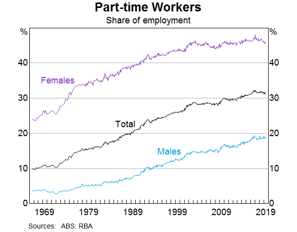
As more people work part time, it has become increasingly common to be both employed and to
work fewer hours than you want to work. In the 1960s, less than one in ten workers worked
part time (Graph 1). Today, one in three of us works part time. Almost one in two women
work part time and more than one in two younger workers work part time.
Graph 1
A few more facts are perhaps helpful here. According to the ABS, around 3 million people
work part time because they want to, not because they can’t find a full-time job. Most
people who are working part time do so because they are studying or have caring
responsibilities, or for other personal reasons. So we should not think of part-time jobs as
being bad jobs, and full-time jobs as being good jobs. Rather, one
of the success stories of the Australian labour market is that we have been able to
accommodate this desire for part-time work and flexibility.
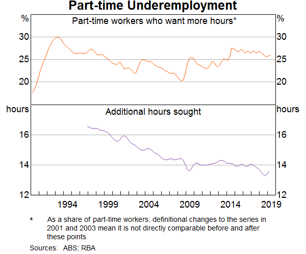
Having said that, around one-quarter of people working part time are not satisfied with the
hours they are offered and would like to work more hours: we can think of these people as
underemployed (Graph 2). The share of part-time workers who are underemployed moves up
and down from year to year, and the current share is above its average level over the past
two decades.
Graph 2
As part of the ABS’s monthly survey of 50,000 people, it asks underemployed workers how
many extra hours they would like to work. On average, they answer that they would like to
work an extra 14 hours per week. It is interesting that this figure has trended down over
the past two decades; it used to be more than 16 hours. Over the same period, the
average hours worked by part-time workers has increased by around 2 hours to 17 hours per
week. Taken together, these data suggest that businesses are doing a better job of providing
the hours that part-time workers are seeking.
This shift to part-time work means that in assessing spare capacity we need to consider
measures of underemployment as well as measures of unemployment. The RBA has
been doing this for some time. As part of our efforts here, we have constructed a measure of
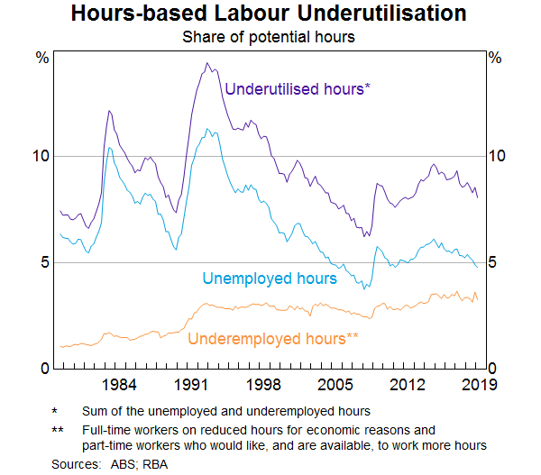
underutilisation that takes account of the part-time workers who want to work more hours.
This measure adds the extra hours sought by these workers to the hours sought by those who
are unemployed (Graph 3).[2]
These extra hours are equivalent to around 3.3 per cent of the labour force,
which, taking account of conventional unemployment, means that the underutilisation rate is
8.1 per cent. This hours-based measure is preferable to heads-based measures of
underutilisation that treats an unemployed person in the same way as a part-time worker
seeking a few more hours.
Graph 3
Unlike the unemployment rate, which has trended down over the past 20 years, the
underemployment rate has been relatively stable. These different patterns in unemployment
and underemployment suggest that fewer inroads have been made into spare capacity in the
labour market than suggested by looking at the unemployment rate alone. This is something we
take into account in thinking about monetary policy.
There is, though, one other perspective on the measure of underemployment that I would like
to share with you. In the past, when part-time work was not as readily available, many
people – mostly women – faced the choice of taking full-time paid employment or
no paid employment at all. Many chose to, or had to stay outside the labour force because
working was not a realistic option. From the perspective of society as a whole, this was a
serious form of underutilisation – it just wasn’t measured as such by the ABS.
Given the trend towards part-time and more flexible jobs, people have more options than they
had before and many have chosen to join, or have deferred leaving, the labour force.[3] From the
perspective of adding to the productive capacity of the nation, this is a good outcome and
if there was a measure of underutilisation that took account of exclusion from the
workforce, it would surely have declined. I don’t want to downplay the issue of
underemployment, but it is worth recognising this broader perspective, and remembering where
we have come from.
Flexibility of the supply side
This naturally brings me to my second window into spare capacity in the labour market –
the flexibility of labour supply.
Over the past 2½ years, the working-age population has increased at an annual rate of
around 1¾ per cent. Over that same time period, employment has increased at
an average rate of 2¾ per cent. The fact that employment has been increasing
considerably faster than the working-age population has led to a reduction in the
unemployment rate, but the reduction is not as large as might have been expected. The reason
for this is that the supply of labour has increased in response to the stronger demand for
workers.
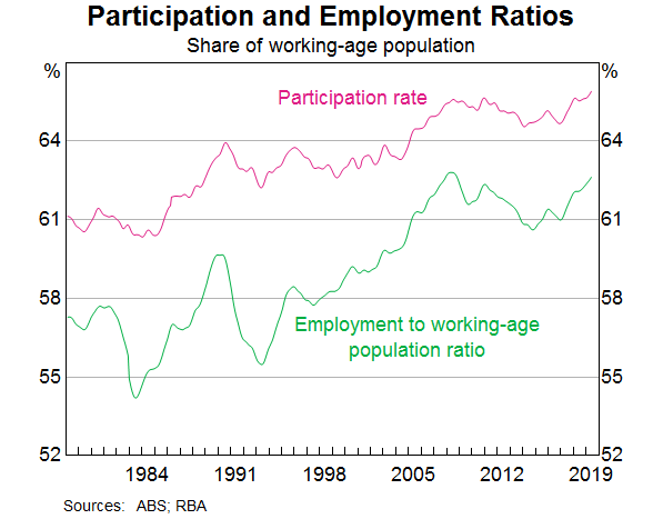
This flexibility in labour supply is evident in the substantial rise in labour force
participation. The participation rate currently stands at 66 per cent, which is
the highest on record (Graph 4). Reflecting this, the share of the working-age
population in Australia with a job is currently around the record high it reached at the
peak of the resources boom. As I discussed a few moments ago, the availability of part-time
and flexible working arrangements is one reason for this.
Graph 4
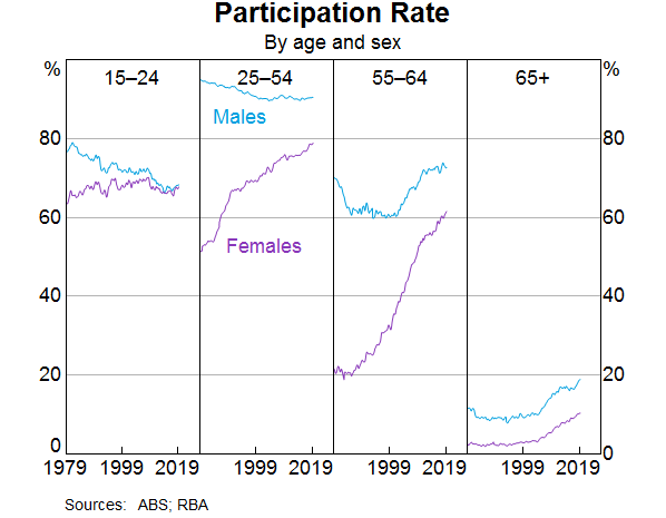
There are two groups for which the rise in participation has been particularly pronounced:
women and older Australians (Graph 5). The female participation rate now stands at 61 per cent,
up from 43 per cent in 1979. Australia’s female participation rate is now
above the OECD average, although it remains below that of a number of countries, including
Canada and the Netherlands.
The participation rate of older workers has also increased over recent decades as health
outcomes have improved and changes have been made to retirement policies. The eligibility
age for the pension was progressively raised from 60 to 65 for females and is now being
gradually increased to 67 for everybody by 2023. The preservation age at which individuals
can access their superannuation is also being gradually increased. These changes are
contributing to higher participation by older Australians.
Graph 5
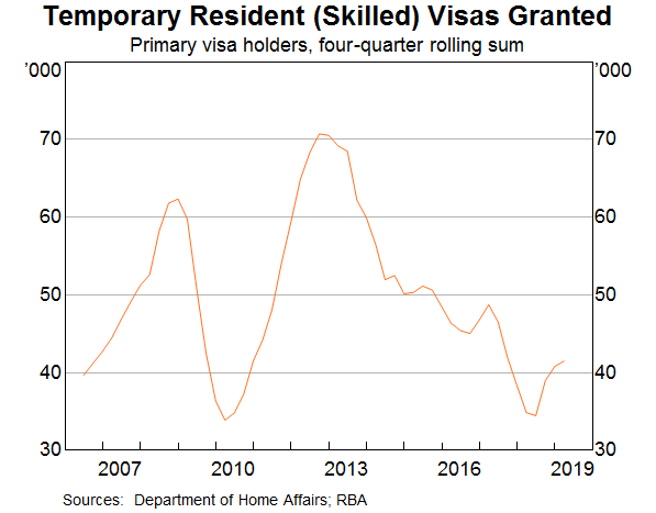
Another source of potential labour supply is net overseas migration. Migration, including
temporary skilled workers, increased sharply during the resources boom when demand for
skilled labour was very strong, and has subsequently declined (Graph 6). While migrants
add to both demand and supply in the economy, they can be a particularly important source of
capacity for resolving pinch-points where skill shortages exist.
Graph 6
A related source of flexibility stems from our unique relationship with New Zealand. When
labour demand is relatively strong in Australia, there tends to be an increase in the net
inflow of workers from New Zealand to Australia. When conditions are relatively subdued
here, the reverse occurs. During the resources boom, the inflow from across the Tasman were
as large as the inflow of temporary skilled workers.
The overall picture here is one of a flexible supply side of the labour market. When the
demand for labour is strong, more people enter the jobs market or delay leaving. This rise
in participation is a positive development. But it is one of the factors that has meant that
strong demand for labour has not put much upward pressure on wages.
The matching of people with jobs
A third perspective on spare capacity in the labour market can be gained from examining how
well people looking for jobs are matched with the jobs that are available. Looking at the
labour market from this perspective, things look a little tighter than suggested by the
other two perspectives that I have discussed.
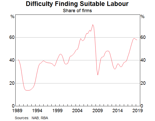
Currently, almost 60 per cent of firms report that the availability of labour is
either a minor or a major constraint on their business (Graph 7). This share is not as
high as it was during the resources boom, but it is still quite high. Reports from the RBA’s
liaison program suggest that there are currently shortages of certain types of engineers,
workers with specialised IT skills and some tradespeople associated with public
infrastructure work. Businesses in regional areas are also more likely to report a greater
degree of difficulty finding suitable labour.
Graph 7
One contributing factor here is an underinvestment in staff training. In the shadow of the
global financial crisis many firms cut back training to reduce costs. We are now seeing some
evidence of the adverse longer-term implications of this. As the labour market tightens
further, I would hope that more firms are prepared to hire workers and provide the necessary
training.
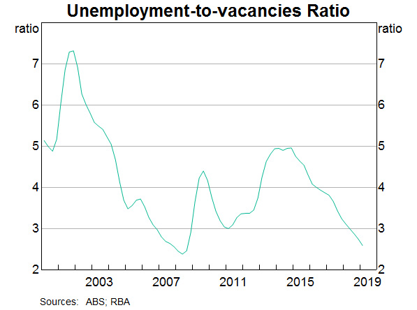
Another lens on job matching is the ratio of the number of unemployed people to the number of
job vacancies (Graph 8). At present, there are fewer than three unemployed people for
each vacancy. This compares with over 20 people for every vacancy in the early 1990s
recession and five people for every vacancy in 2014. From this perspective the labour market
looks reasonably tight. There is also some tentative evidence that, on average, unemployed
workers are not as well matched to job vacancies as was the case in 2007, when the ratio of
the two was at a similar level.
Graph 8
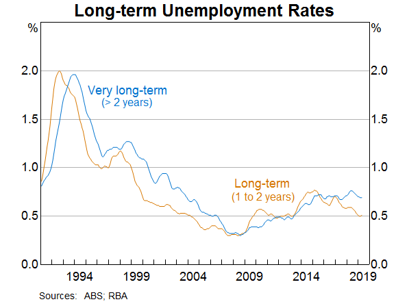
One such piece of evidence is that as the unemployment rate has come down over recent years,
there has been little progress on reducing very long-term unemployment, defined as those who
are unemployed for more than two years (Graph 9). Addressing the causes of this chronic
unemployment remains an important challenge for our community. More positively, the share of
the labour force that has been unemployed between one and two years has trended down over
recent times.
Graph 9
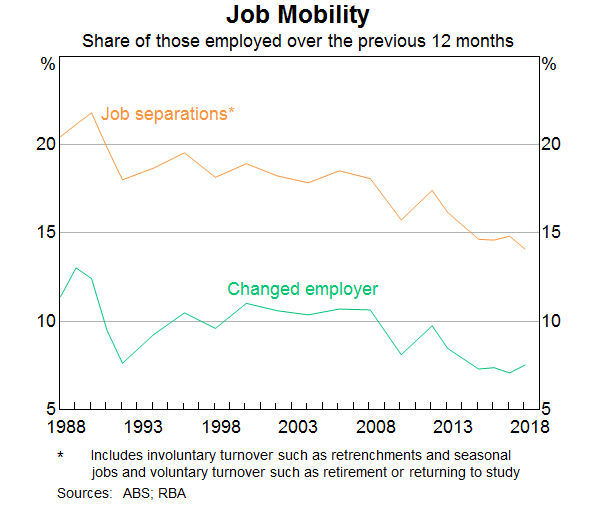
Another lens on job matching and the overall tightness of the labour market is the rate of
job mobility; that is, how often people change their jobs. Here, the evidence is
interesting. Despite the frequent reports of a lack of job security and regular job
switching by millennials, the average time that workers are staying with an employer is
increasing. Reflecting this, the share of employed people who switch employers in a given
year is the lowest it has been in a long time (Graph 10). Looking at the data by
occupation, the rate of job mobility is lowest for managers and business professionals and
highest for tradespeople and workers in the hospitality industry.
Graph 10
In a tight labour market, we would expect to see either strong wages growth or frequent job
changing as businesses seek out workers. But we are seeing neither at present. One possible
explanation for this is the uncertainty that many people feel about the future. This
uncertainty means that if you have a job you want to keep it rather than take a risk with a
new employer. This might be especially so if you also have a large mortgage. So it is
possible that the high level of household debt is also affecting labour market dynamics.
Wages
I will now turn to the fourth perspective on labour market tightness – that is wages
growth.
Over the past year, wages growth has picked up as the labour market tightened. This is not
surprising given the strength of demand for labour. But the pick-up has been fairly modest
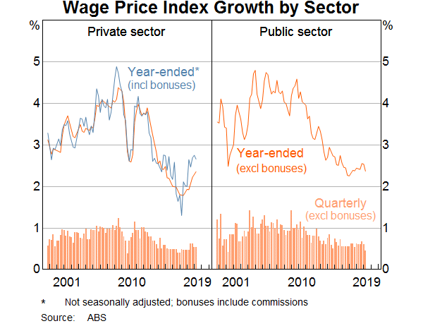
and is only evident in the private sector (Graph 11). Over the past year, the
private-sector Wage Price Index increased by 2.4 per cent, up from 1.9 per cent
in the previous year. The past two quarters have, however, seen lower wage increases than in
the previous two quarters.
In contrast to trends in the private sector, wages growth in the public sector has been
steady at around 2½ per cent, largely reflecting the wage caps across much of
the public sector.
It is also worth pointing out that overall wages growth in New South Wales and Victoria has
been running at just 2½ per cent despite the unemployment rate being 4½ per cent
or lower over the past year.
Graph 11
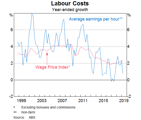
Another perspective on wages growth is from the national accounts, which reports average
earnings per hour worked (Graph 12). This measure is volatile, but the latest data
painted a fairly weak picture, with average hourly earnings up by just 1 per cent
over the past year.
Graph 12
In summary, the overall picture from these various windows into the labour market is that
despite the strong employment growth over recent times, there is still considerable spare
capacity in the labour market. We remain short of the unemployment rate associated with full
employment, there is significant underemployment and there is further potential for labour
force participation to increase when the jobs are there. Consistent with all of this, wages
growth remains modest and is below the rate that would ensure that inflation is comfortably
within the 2 to 3 per cent range. The one caveat to this assessment is the
difficulty that some firms are having finding workers with the necessary skills. This
underlines the importance of workplace training.
Monetary Policy
I would like to finish with a few words on monetary policy.
As you are aware, the Reserve Bank Board reduced the cash rate to 1¼ per cent
at its meeting earlier this month. This was the first adjustment in nearly three years.
This decision was not in response to a deterioration in the economic outlook since the
previous update was published in early May. Rather, it reflected a judgement that we could
do better than the path we looked to be on.
The analysis that I have shared with you today supports the conclusion that the Australian
economy can sustain a higher rate of employment growth and a lower unemployment rate than
previously thought likely. Most indicators suggest that there is still a fair degree of
spare capacity in the economy. It is both possible and desirable to reduce that spare
capacity. Doing so will see more people in jobs, reduce underemployment and boost household
incomes. It will also provide greater confidence that inflation will increase to be
comfortably within the medium-term target range.
Monetary policy is one way of helping get us onto to a better path. The decision earlier this
month will assist here. It will support the economy through its effect on the exchange rate,
lowering the cost of finance and boosting disposable incomes. In turn, this will support
employment growth and inflation consistent with the target.
It would, however, be unrealistic to expect that lowering interest rates by ¼ of a
percentage point will materially shift the path we look to be on. The most recent
data – including the GDP and labour market data – do not suggest we are making
any inroads into the economy’s spare capacity. Given this, the possibility of lower
interest rates remains on the table. It is not unrealistic to expect a further reduction in
the cash rate as the Board seeks to wind back spare capacity in the economy and deliver
inflation outcomes in line with the medium-term target.
It is important though to recognise that monetary policy is not the only option, and there
are limitations to what can be achieved. As a country we should also be looking at other
ways to get closer to full employment. One option is fiscal policy, including through
spending on infrastructure. Another is structural policies that support firms expanding,
investing, innovating and employing people. Both of these options need to be kept in mind as
the various arms of public policy seek to maximise the economic prosperity of the people of
Australia.
The latest from the UK suggests inflation will fall below the 2% lower bounds as downside risks to growth build and the Brexit issue still haunts the halls. The Bank held the current rate, and will continue its market operations to stimulate the economy.
The Bank of England’s Monetary Policy Committee (MPC) sets monetary policy to meet the 2% inflation target, and in a way that helps to sustain growth and employment. At its meeting ending on 19 June 2019, the MPC voted unanimously to maintain Bank Rate at 0.75%.
The Committee voted unanimously to maintain the stock of sterling
non-financial investment-grade corporate bond purchases, financed by the
issuance of central bank reserves, at £10 billion. The Committee also
voted unanimously to maintain the stock of UK government bond purchases,
financed by the issuance of central bank reserves, at £435 billion.
The MPC’s most recent economic projections, set out in the May Inflation Report,
assumed a smooth adjustment to the average of a range of possible
outcomes for the United Kingdom’s eventual trading relationship with the
European Union and were conditioned on a path for Bank Rate that rose
to around 1% by the end of the forecast period. In those projections,
GDP growth was a little below potential during 2019 as a whole,
reflecting subdued global growth and ongoing Brexit uncertainties.
Growth then picked up above the subdued pace of potential supply growth,
such that excess demand rose above 1% of potential output by the end of
the forecast period. As excess demand emerged, domestic inflationary
pressures firmed, such that CPI inflation picked up to above the 2%
target in two years’ time and was still rising at the end of the
three-year forecast period.
Since the Committee’s previous meeting, the near-term data have been
broadly in line with the May Report, but downside risks to growth have
increased. Globally, trade tensions have intensified. Domestically, the
perceived likelihood of a no-deal Brexit has risen. Trade concerns have
contributed to volatility in global equity prices and corporate bond
spreads, as well as falls in industrial metals prices. Forward interest
rates in major economies have fallen materially further. Increased
Brexit uncertainties have put additional downward pressure on UK forward
interest rates and led to a decline in the sterling exchange rate.
As expected, recent UK data have been volatile, in large part due to
Brexit-related effects on financial markets and businesses. After
growing by 0.5% in 2019 Q1, GDP is now expected to be flat in Q2. That
in part reflects an unwind of the positive contribution to GDP in the
first quarter from companies in the United Kingdom and the European
Union building stocks significantly ahead of recent Brexit deadlines.
Looking through recent volatility, underlying growth in the United
Kingdom appears to have weakened slightly in the first half of the year
relative to 2018 to a rate a little below its potential. The underlying
pattern of relatively strong household consumption growth but weak
business investment has persisted.
CPI inflation was 2.0% in May. It is likely to fall below the 2%
target later this year, reflecting recent falls in energy prices. Core
CPI inflation was 1.7% in May, and core services CPI inflation has
remained slightly below levels consistent with meeting the inflation
target in the medium term. The labour market remains tight, with recent
data on employment, unemployment and regular pay in line with
expectations at the time of the May Report. Growth in unit wage costs
has remained at target-consistent levels.
The Committee continues to judge that, were the economy to develop
broadly in line with its May Inflation Report projections that included
an assumption of a smooth Brexit, an ongoing tightening of monetary
policy over the forecast period, at a gradual pace and to a limited
extent, would be appropriate to return inflation sustainably to the 2%
target at a conventional horizon. The MPC judges at this meeting that
the existing stance of monetary policy is appropriate.
The economic outlook will continue to depend significantly on the
nature and timing of EU withdrawal, in particular: the new trading
arrangements between the European Union and the United Kingdom; whether
the transition to them is abrupt or smooth; and how households,
businesses and financial markets respond. The appropriate path of
monetary policy will depend on the balance of these effects on demand,
supply and the exchange rate. The monetary policy response to Brexit,
whatever form it takes, will not be automatic and could be in either
direction. The Committee will always act to achieve the 2% inflation
target.